Lab 7: Census Data Analysis and Geocoding
Xiaozhong Sun
2023-05-07
Due Date: March 22th
Instructor: Xiaozhong Sun (xs243@cornell.edu)
Lab TAs: Wenzheng Li (wl563) / Ishan Keskar (iuk3) / Aditi Parihar [ap973@cornell.edu]
Location: Sibley 305, Barclay Gibbs Jones Computer Lab
Total Points: 100
Goals for this lab
This week’s lab contains three goals:
The first goal is utilizing GIS to undertake census level data analysis. Reinforce what you have learn from previous lab. In this exercise, we will utilize GIS to explore and document issues of environmental justice in Massachusetts. You will required to answer the following questions:
- What is the relationship between race and proximity to locally unwanted land uses?
- Are certain segments of the population disproportionately impacted?
The second goal is about geocoding using coordinates vs. addresses. You will download two datasets, one on crime complaints, one on business operations, from NYC Open Data and try to geocode them.
The third goal is learning integrate ArcGIS Pro and Google Earth Pro, you will learn how to create your own spatial data from KML file.
Census Data Case Study
Now, compare and contrast the African American population living within 1 mile of landfills for the Boston metropolitan area. In defining the metropolitan Boston spatial extent, utilize the boundary of Regional Planning Agency.
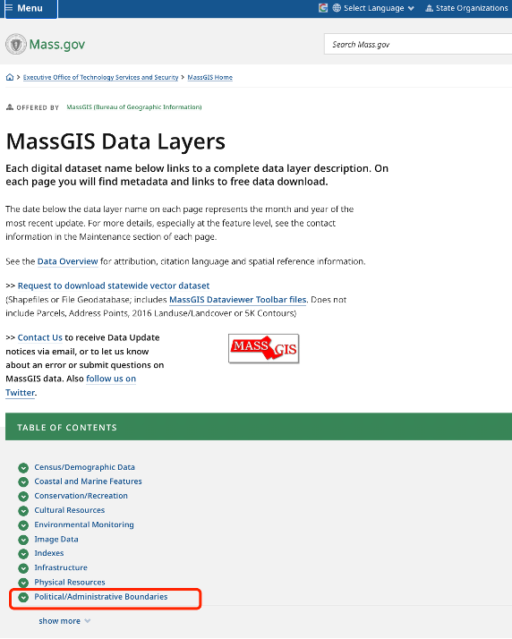
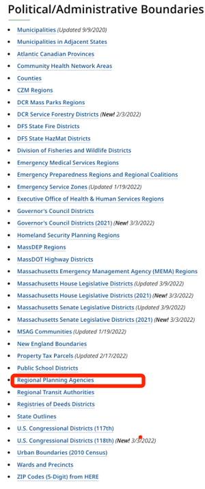
- Go to https://www.mass.gov/info-details/massgis-data-layers, and expand the layer under ‘Political/Administrative Boundaries’.
- It will redirect you to a new page called ‘MassGIS Data - Regional Planning Agencies.’
- Download the data.
Before you refer to the demo below. I think this is a great opportunity for you to think independently about how to do a complex GIS spatial analysis, using the techniques we learned earlier. Try to write down critical steps for you to finish this task. Solving complex spatial analysis will also be an essential ability for you to complete your final project independently.
Tasks:
- Calculate the population percentage African American for the Boston Metro area.
- Calculate the percentage of population living within 1 mile of landfills that is African American in the Boston metropolitan area. Do African American in Boston tend to be disproportionately concentrated around landfills compared with their metro-wide population percentage?
- Compare this with the percent of African American statewide.
Demo
To undertake this analysis, we will need several datasets:
- State boundary files (census tract boundaries),
- the Boston metropolitan area boundary file downloaded from the previous steps,
- Demographic or race data aggregated to census tracts, and
- Point data for locally unwanted land uses (landfills).
Moreover, in order to determine whether the impact is disproportionate to a specific population, we will need some sort of benchmark with which to compare our findings and conduct our analysis. In this case, we will compare our findings to the state level data.
To undertake the analysis, we will calculate the percentage of the population living within 1 mile of a landfill that is African American. We will then compare this to the statewide African American population percentage.
As our population data is aggregated through enumerated units identified by the Census Bureau, and not according to distance from landfills, we will have to undertake some geoprocessing before completing our analysis.
Often state governments or public agencies will compile a range of data sets that are relevant to the state and make this data publicly available through a GIS repository. This is often helpful, particularly if we require data from different sources that must be integrated, as the data has already been formatted accordingly. For this lab, we will utilize data made available by the state of Massachusetts.
- https://www.mass.gov/info-details/massgis-data-layers. Take a look at the available datasets.
- Scroll to “Census/Demographic data”
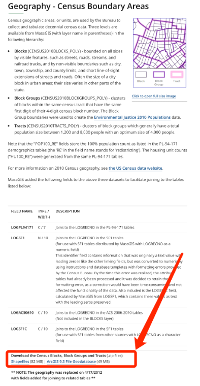
- Click on “Data layers from the 2010 US Census.” You will be redirected to a new page.
- Download the Census Tracts shapefile available under ‘Geography –
Census Boundary Areas.’
- Note that some users click a download data link and nothing happens. This is a browser security issue that can be overcome in several ways. Either try a different browser or right-click the download link and use one of the “Save As” options in the dropdown menu.
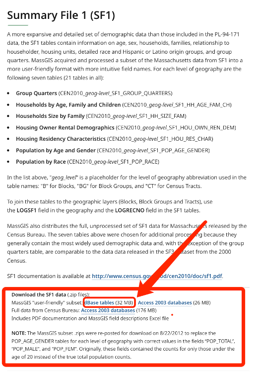
- Download Summary File (SF1) dataset available on the same page.
Now go to the Canvas, download and unzip the Lab 7 data. Find the folder “solidwaste”.
There are a number of datasets included in the zip files, but the one we are interested in is the Solid Waste Land Disposal point data layer (SW_LD_PT), compiled by the Massachusetts Department of Environmental Protection (DEP) to track the locations of land disposal of solid waste. Please be sure you read some of the information associated with each dataset, so you know how you are to utilize them in ArcGIS.
Open ArcGIS Pro. Add the Census Tracts. Note that they are already projected (State_Plane_Massachusetts_Mainland), however, please note that the map units being used are meters. It is only convention that associates State Plane with feet. If you open the attribute table, note that the area is recorded in square feet. Therefore, all units related to area should be square feet when you do the calculation and generate new field.
Add the appropriate SF1 database containing population and race data, i.e., CEN2010_CT_SF1_POP_RACE. Again, be sure you are utilizing tract level attribute information, not blocks or block groups).
Please join the SF1 database to the 2010 Census Tracts. Look at the attribute tables and/or metadata to determine the appropriate join fields.
Add the Solid Waste Land Disposal point layer (SW_LD_PT).
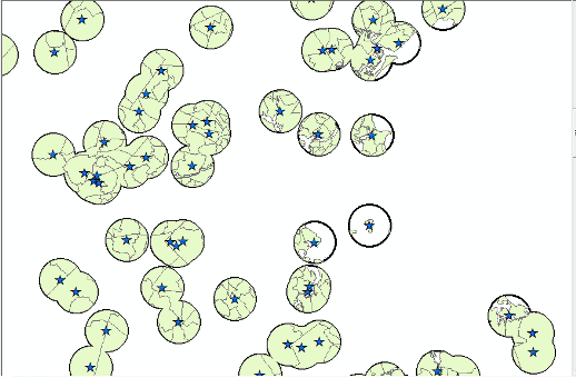
Open the Buffer tool (Analysis/Buffer). Set the input to the Landfill shapefile. Name the output and be sure to send it to your output folder. Set the buffer distance to 1 mile. Select ‘Dissolve all output features into a single feature’ as the Dissolve type. Click Run.
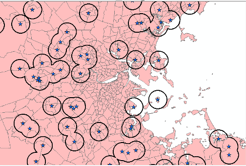
Clip the census tracts to the dissolved buffer layer. Set the output location and name. Click Run. You will recall that the clip function does not affect the original attribute information, therefore, you need to calculate the geometric using steps from previous lab. (if we were operating within a Geodatabase it would, but you shouldn’t save it to Geodatabase.).
Zoom in briefly, and using the identify tool, toggle on and off the original Census tract layer and your newly created clipped tract layer. Notice that the attributes for the clipped census tracts are the same as those original census tract (as a point of comparison, check out the AREA_SQFT field).
We will need to calculate the new areas of the clipped polygon census tracts.
Open the Attribute table of the clipped census tract layer.
- Click Add.
- Name the field ‘NewArea’, set the data type to “Double” and number format to “Numeric”. Click Save.
Right-click on the field NewArea —> Calculate Geometry.
- Set the Property to Area.
- Set the appropriate unit (Square feet) for the “NewArea.”
- Click Run. Close the attribute table.
Based on the relative proportion of each census tract that lies within the 1-mile buffer we have delineated; we will now estimate the population that is African American (use the ‘pop_black’ variable for the African American totals).
- In the clipped census tract shapefile attribute table > Attribute table > Add Field. Name it ‘Popblk_cl’ or something similar, set the type to “Double” and Number format to “Numeric”. Click Save.
Right-click on the field ‘Popblk_cl’ > Calculate Field (Note: different from Calculate Geometry). Make sure you have started editing.
- Write a formula to calculate the population that is black within our buffer. Click Run.
Note: This spatial analysis is not perfect. We basically assume that the population within the census tract is evenly distributed, which is not entirely true. However, suppose the buffer of the landfills covers a large portion of the census tract. In that case, it is reasonable to infer that the majority of the population within the tract is affected.
Now it’s your turn!!!
Referring to the Demo, answer Questions 1-5 (55 points).
Recall the tasks’ requirements:
- Calculate the population percentage of African American for the
Boston Metro area.
- Note that: to identify those tracts within the regional boundary, please obtaining the Boston Metro census tract layer by selecting the census tracts that had their centroid within the Boston metro area. Do not simply clip. [Recall what we have learned previously, using select by location!]
- The most accurate results should also include the Boston island census tracts. With the newly updated data, the Boston metro polygon layer should already includes these island census tracts. If not, you can add them by using additional geoprocessing tools.
- Calculate the percentage of population living within 1 mile of landfills that is African American in the Boston metropolitan area. Do African American in Boston tend to be disproportionately concentrated around landfills compared with their metro-wide population percentage?
- Compare this with percentage of population that is African American statewide.
Note: for all the numbers you will answer below, DO NOT keep for more than 2 decimal places.
Question 1 (10 points):
Calculate the population percentage of African-American for the Boston Metro area.
Question 2 (5 points):
What formula did you use to calculate the population that is African American within the 1-mile buffer? Write down both the mathematical formula and Query formula you constructed in ArcGIS Pro.
- Hint: You can assume that the ratio of African American within 1-mile buffer to the total African American is equal to the ratio of NewArea (within Buffer) to the total Area. Assuming population is evenly distributed across the space.
Question 3 (10 points):
Now you should have the total African American population (count) living within 1-mile buffer of landfills. What percent of population living within 1 mile of landfills that is African American?
- Hint: You need first calculate the total population living within the 1-mile buffer of landfills.
Question 4 (10 points):
How does this percentage compare to the statewide percentage of African American population? (10 points).
- Hint: use the original census tracts layer (with 1472 features) rather than the clipped layer to calculate percentage population statewide.
Question 5 (10 points):
What are your conclusions concerning the spatial distribution of African Americans in Massachusetts in relation to landfills?
Question 6 (10 points):
What are some of the weaknesses of this approach, particularly in terms of accuracy? (5 points)
How could you undertake a more accurate spatial analysis? (5 points)
Geocoding
In this part, you will geocode and map all the crime complaint data in NYC happened during June 2022 by their
- coordinates and
- addresses.
Geocoding by XY coordinates
- Go to NYC Open Data Portal (https://opendata.cityofnewyork.us/)
- Use “crime” as the keyword to search for crime-related dataset
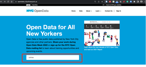
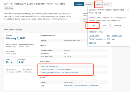
- Find the “NYPD Complaint Data Current (Year To Date)”
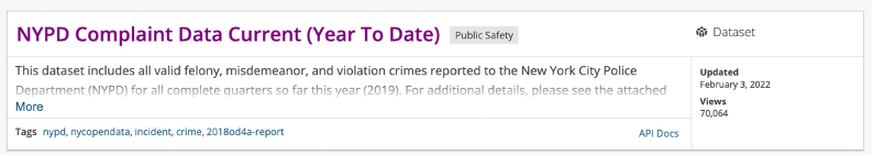
- Go to the data page, explore what kind of data and supporting files
are provided.
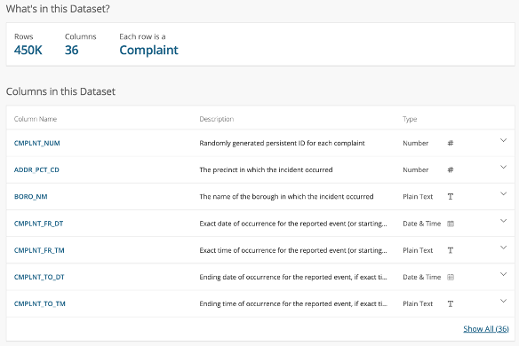
- This page provides your all crime complaints up till the most recent date in NYC, more than 500K rows, with 36 columns, a kind of “big data” set you handle so far.
- The attachments are supporting files to explain the data structure, variable names, and data collection methods.
- Go to Export –> CSV and download the CSV file.
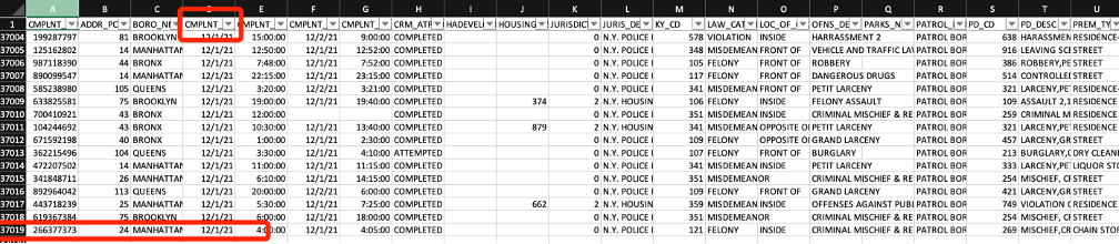
- Open the CSV file, manually clean it by selecting only the
June in 2022, save it as a .csv file.
- You can activate “Data->Filter” function in Excel, filter the dataset by CMPLNT_FR_DT column to June 2022
- Save the data (as CSV again), you will now have about 46980 rows of
complaint records
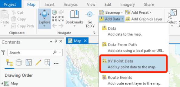
- Import the new and clean June dataset in ArcGIS Pro, map the dataset
by coordinates, using
Map–>Add Data–>XY Point Datafunction.- Set the coordinates accordingly (X: longitude, Y: Latitude, Coordinate System: your choice)
- Click “Run”, it might take a few seconds.
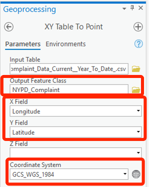
- Once completed, you will see a new layer with corresponding complaint data points similar to this one.
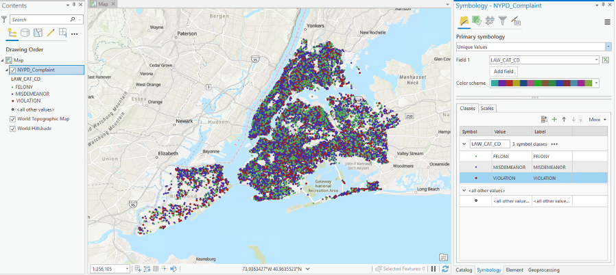
Now it’s your turn!!!
Generate a map layout, visualize the data by “LAW_CAT_CD” column (categorical) with readable legend settings (10 points).
Now commenting one whether using point data is helpful for describing the crime complaint in NYC. Can you find certain spatial patterns? What would you do to improve the interpretability using this data set? Write down the additional spatial data and ArcGIS operations you might use. (10 points).
Geocoding by addresses
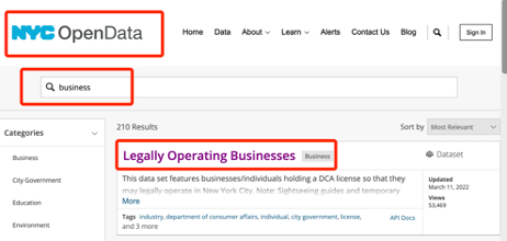
- Go to NYC Open Data and search for “business” related dataset.
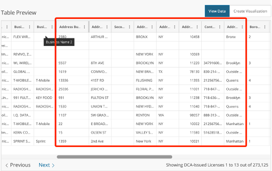
- Go to the “Legally Operating Businesses” page, browse the data variables, note that how the full addresses are coded by several columns.
- Download this data in csv format, open it in excel, choose only 10 rows of the data with complete address information, and save it (some data don’t have a full record of address information, remember only filter businesses within NYC).
- Import the only-10-row csv new data (your choice of ten records)
(Legally_Operating_Businesses.csv) using
Data–>Add Datato ArcGIS Pro as a table. - Right click to open attribute table. Look for what columns contain addresses to be geocoded?
- Right click and use “Geocode Table” to geocode the addresses to a map, see what’s different from that of geocoding by coordinates.
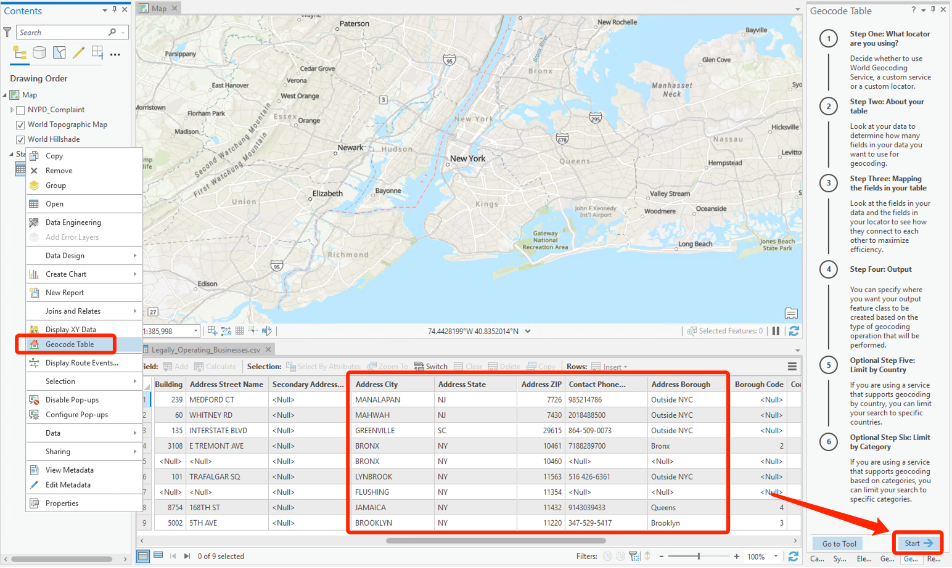
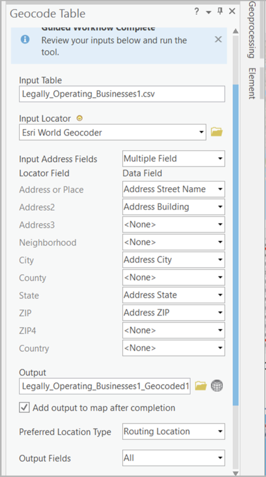
- Step 1: Choose Esri World Geocoder as the Input Locator
- Step 2: Make sure the correct table, and “More than one field” are selected
- Step 3: Set the addresses by selecting columns, continue to Step 4-6 until you reach the “Run”
- Double-check all settings, and “Run” it.
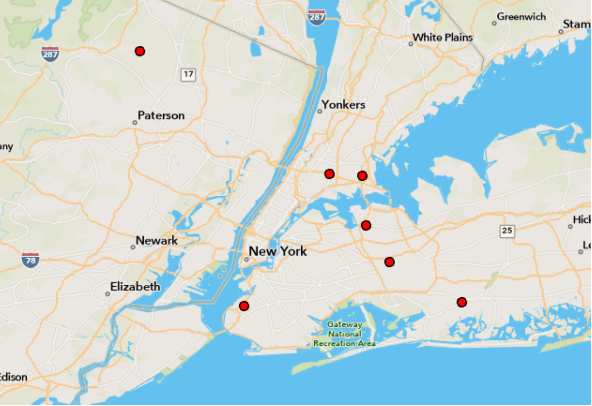
- Theoretically, you should be able to create a map with the business
data (similar like the map below). However, you might not be able to get
the map for this time, because the CU account might not provide geocoding
credit, therefore you might not be able to get the results properly.
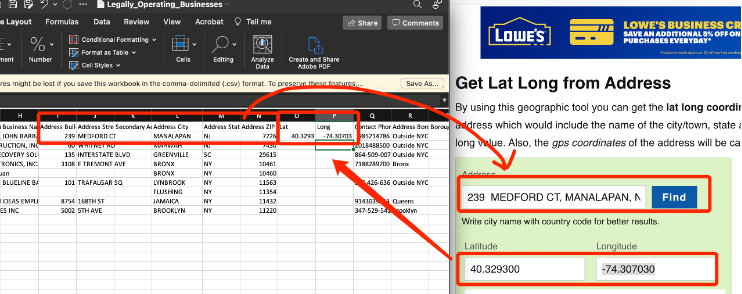
- What should we do? Don’t worry, there are many online and free Lat
Long converters (A new way of DIY geocoding).
- For example, visit this one (https://www.latlong.net/convert-address-to-lat-long.html)
- Generate the (lat, long) coordinates manually, and copy and paste them to the columns of longitude and latitude if there are no records in the csv file, save the .csv with lat and long information for the new addresses.
Now it’s your turn!!!
If you cannot use the geocoding credit provided by the ArcGIS Pro, use the new csv (come with full records of coordinates that you manully acquired), geocode the dataset with longitude and latitude data. Make a map layout with readable legends and layouts (10 points)
- Please describe/criticize the geocoding process using “addresses vs coordinates”, which do you prefer? Which is more convenient? What should we pay attention to during the workflow of geocoding using addresses? What will determine the accuracy of the results? (5 points)
ArcGIS Pro and Google Earth Pro
What if we want to generate a layer to show grocery stores in Ithaca, but we don’t have either x,y coordinate or location information for the grocery stores? Yes, we can use Google Earth to generate locations for grocery stores! This gives us another option for geocoding spatial data.
In the following part, we will explore how to export a location or data from Google Earth. This can be very helpful when you want to generate location data that is not available out there.
The target of this exercise is to draw a map shows the location of grocery stores in the City of Ithaca. However, currently we don’t have any location information about those stores.
We will need to use Google Earth Pro to generate the locations of grocery stores and then import the information into ArcGIS Pro.
We will use data format KML (Keyhole Markup Language) which is the data format that Google Earth uses. Then convert the KML file to shapefile. From there we can either make a map or conducting spatial analysis.
Exporting files from Google Earth to ArcGIS
- Download Google Earth Pro. https://www.google.com/earth/versions/
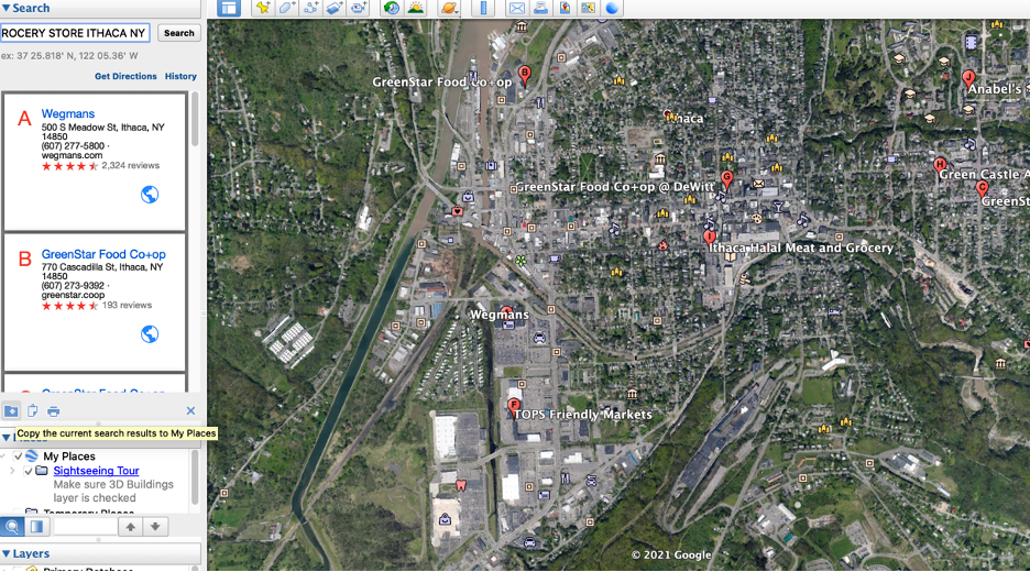
- Search grocery stores in Ithaca, NY.
- Copy the current search results to my places,
click

- You will see that, there is a new file “grocery store Ithaca ny” generated under My Place tab.
- Right click “grocery store Ithaca ny” file and then click “save place as.” Give the file a name grocerystores, and place in your folder. You can see that the file type is kmz/kml file. That’s the format of Google Earth data. You have now exported a kmz/kml file.
Open ArcGis Pro. Within the Conversion toolbox, go to
KML toolset and KML To Layer. This tool creates a file
geodatabase containing a feature class within a feature dataset.
The Dialogue box will ask you to navigate to the kml file and select an output location. Please note that it wants you to place the output within a folder, so be sure to select an actual folder as your output!
You can also specify an output data name. Once you have converted your kml to layer process, it should automatically be added to your map.
Check the attribute table of this point layer. You can see that it contains address information, as well as store name information which is exported from Google Earth.
The Output will be generated in the WGS84 coordinate system (default GCS of Google Earth). We are working on locations in NY, so change the projection of your map to State Plane New York Central.
Note: you will need to change the projections of both your data frame and the grocerystores layer. If you don’t change the projection of your data frame from WGS 1984 to state plane, even though the layer is changed to state plane, it will still be displayed in the projection of WGS 1984. (Again, remember projection on the fly from lab 3 🤓?)
To change the projection of your grocerystores layer, use
Project. (Note: still remember the difference between
define projection and project?)
Want to get hands on more awesome open geo-data? Check out this tutorial on Youtube.
Now it’s your turn!!!
Create a layout of the grocery stores in the city of Ithaca. Add an appropriate basemap to show the context information. Label the grocery store names on your map. (10 points)
The END