Lab 6: Census Data Preparation and Management
Xiaozhong Sun
2023-05-07
Due Date: Mar 15 th
Instructor: Xiaozhong Sun (xs243@cornell.edu)
Lab TAs: Ishan Keskar [iuk3@cornell.edu], Aditi Parihar [ap973@cornell.edu]
Location: Sibley 305, Barclay Gibbs Jones Computer Lab
Total Points: 110
Goals for this lab
In this lab, you will be instructed to explore different data sources for preparing your own research project.
- You will learn how the Modifiable Areal Unit Problem (MAUP) affects the distribution of a variable across space;
- You will also learn to combine shapefile data with additional attribute data in ArcGIS Pro.
Notes before you start:
- If you export a table from ArcGIS and wish to open it in Excel, ArcGIS creates 2 files (a .dbf and a .xml). You want to be sure to open the .dbf file!
- Please review the deliverable requirements before the Demo to gain an understanding of what will need to be produced from the exercise.
- There is no prepared data for this lab, all data is downloaded from the websites.
- Please make sure you register an account for IPUMS before working on this lab.
Understanding the Census Data and its Hierarchy
Census data is a important data source goes hand-in-hand with the well-defined statistical or political boundaries in GIS analysis. It is important to be able to analyze census information at the municipal, tract, block group and block level, particularly when looking at things like demographic change.
Census Tracts are comprised of several (or maybe one) Block Groups, depending on population density. Each Block Group is composed of Blocks. Blocks are the smallest scale for which census information is available. Blocks are generally coterminous with actual street blocks. For a diagram of the standard census geographic hierarchy, check out this document of U.S census.
Due to confidentiality rules, some fields of census data are not available at the block level, but all the basic count information used for redistricting (a revision of Congressional Boundaries to reflect changes in population) is available at the block level.
To undertake our analysis, we need two things:
- a source for the boundary files (geographic data) and
- a source for the census (attribute/table) data.
What we will do is we will join the appropriate attribute data to our geographical units to conduct any spatial analysis. We will discuss three sources of census data:
- New York State geospatial repository,
- The Federal census website, and
- A private vendor.
Accessing data via CUGIR
We will first explore local data using the Cornell University Geospatial Information Repository (CUGIR), which has already combined both attribute information and boundaries for you.
A quick glance demonstrates that the Cornell University Geospatial Information Repository hosts many datasets of interest to anyone working in the state. For this exercise, we will focus exclusively on accessing census data. Census blocks, block groups and tracts are available for 1990, 1995, and 2000.Please note that most states maintain similar geographic information repository with access to many states, county, and local datasets, usually hosted through a state agency, such as the Department of Environmental Conservation, or other publicly funded institution. These are easy enough to find through googling.
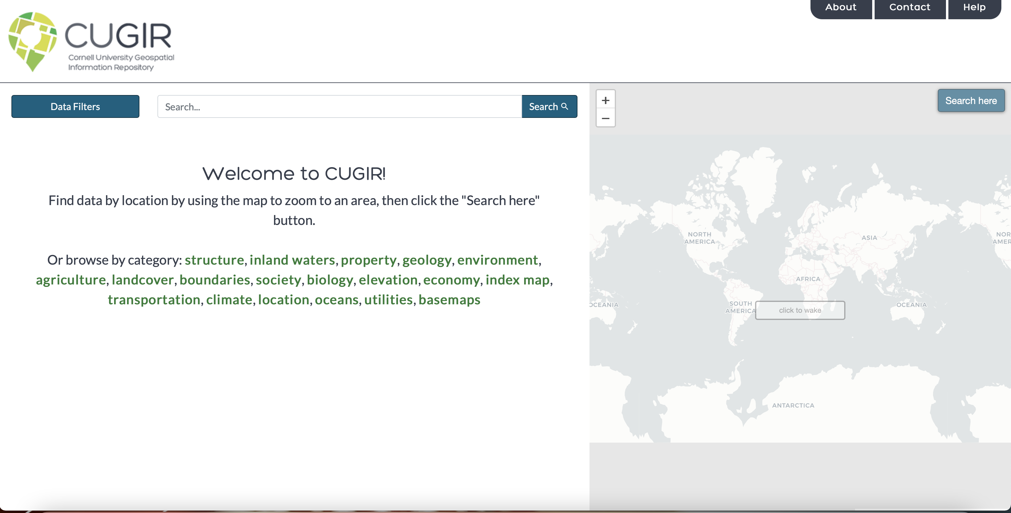
Click Data Filters from the menu bar and then examine
some of your options. We can explore the available data by category,
year, author, collection, place, and data type. Familiarize yourself
with some of the available options.
Under Category, click Boundaries. Note how
the data is organized. Search for New York in the search box.
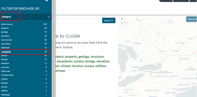
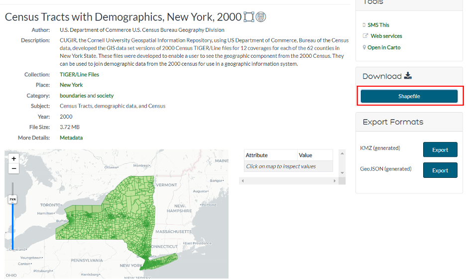
- For our purposes, search for Census Tracts with Demographics, New York, 2000.
- Note how the information is presented – the description contains some basic information about the data, the subject, the author, the year etc.
Under Download on the right-hand side, select ‘Shapefile’. Start ArcGIS Pro, add your new shapefile. We know that the FIPS code for Tompkins County is 109 (See https://transition.fcc.gov/oet/info/maps/census/fips/fips.txt for reference).
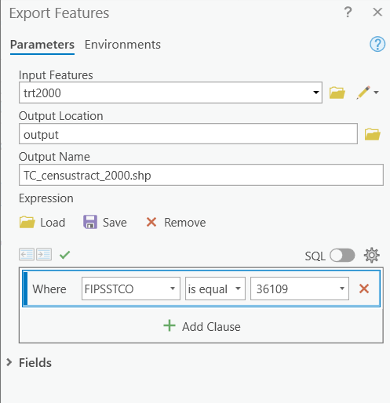
We will now build a query to select all census tracts of Tompkins County and export to a new shapefile.
- Right click the census tract layer and click “Data/Export
Features.”
- Add a new expression.
- We can select by FIPSSTCO. The state FIPS code for NY is 36, so the FIPSSTCO value for Tompkins County is 36109.
- Build a query ‘“FIPSSTCO” = ’36109’’.
- We have now selected all census tracts within Tompkins County.
- Rename it as TC_censustract_2000 and Export it into a new shapefile
Open the attribute table of TC_Censustracts_2000 and take a look at the available information.
This is the same array of data that was available in the thematic map lab. These are referred to as SF1 variables (more on this below). If you look at the projection information you will note it is Geographic Coordinates System (Decimal Degrees). Since we are creating New York state maps, however, we should be sure to project this to New York State Plane!
Now download Census Block Groups with Demographics, New York, 2000 and Census Blocks with Demographics, New York, 2000, then create shapefiles for Tompkins County using the same methods.
Tasks:
Create the following three projected maps (be sure to include projection information, data source, and a color classification as part of the notes on each map here and the following maps).
Compare and contrast them in terms of the MAUP (modifiable areal unit problem).
Map 1: Create a layout of normalized African American population (2000) for Tompkins County with a classification of your choice at the Census Tract level.
Map 2: Create a layout of normalized African American population (2000) for Tompkins County with a classification of your choice at the Block Group level.
Map 3: Create a layout of normalized African American population (2000) for Tompkins County with a classification of your choice at the Block level.
Question #1: Discuss how differences in the unit of analysis affects spatial patterns (5 points)
Creating a new field
Let’s say we wish to normalize instead by 1000 population, in order to standardize our comparisons. This will eliminate the need for ratios, percentages, etc. and allow for easier whole number comparisons between states. We will now create new data by adding a new field.
Open the attribute table for Tompkins County census tracts. Click on
the Add
button
Double
in the Data Type field. Select Numeric and leave 2 decimal
places in the Number Format field. Hit Save to apply the changes.
Now that we’ve created a field, we need to create data to populate
the field. This requires editing. Be sure the editor tab is
present.
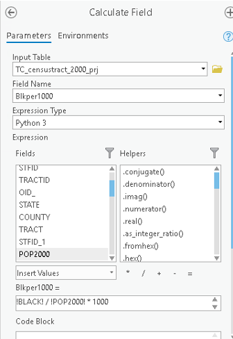
Back in the attribute table, right click on the new field you created
‘Blkper1000’ and go to Calculate Field. Note that field
calculator dialog box contains a listing of all the available fields,
and below this is a query builder box. There are also a series of
operations available.
Enter the query to determine African American population per 1000. To enter the variables, double-click on the fields BLACK and POP2000 to enter them in the query builder box.
Tasks:
- Map 4: Create a layout of African American population (2000) per 1000 for Tompkins County with a classification of your choosing at the Census Tract level. Note that the African American population (2000) per 1000 should be shown in whole number in the legend.
Now, select the census tracts with a majority (over 50%) of renter-occupied housing units. Create a new field “renter_maj” depicting the percentage of renter occupied housing units per 100 housing units (in other words, a percentage). Enter the appropriate formula in the “Calculate Field” to calculate the percentage of renter occupied housing each census tract (use HSE_UNITS). Next, export to a new shapefile the census tracts with a majority (over 50%) of renter-occupied housing units. We should know how to write the formula in the Expression.
Export the selected census tracts to your folder and give it an appropriate filename. Save your project.
- Map 5: Create a map layout that zooms into the census tracts with a majority (over 50%) of renter-occupied housing units. Include a context map as well. Make sure that each tract is labeled with its Tract_ID value.
Sources for Data Collection
Downloading boundary files
An important part of data management in spatial analysis is you can collect additional data and join them with your shapefile data in ArcGIS. This means before we do the data join, we need to download the desired shapefile data and the tabulate data somewhere.
Besides the CUGIR we mentioned above (you might notice the data hosted by CUGIR is somewhat outdated), another popular place to download shapefile boundary data is from the US Census Bureau website. It contains cartographic boundary files, including census tracts, block groups, and blocks, as well as many other sub-divisions at the state and county level. (Of course you can always find shapefiles by search online.)
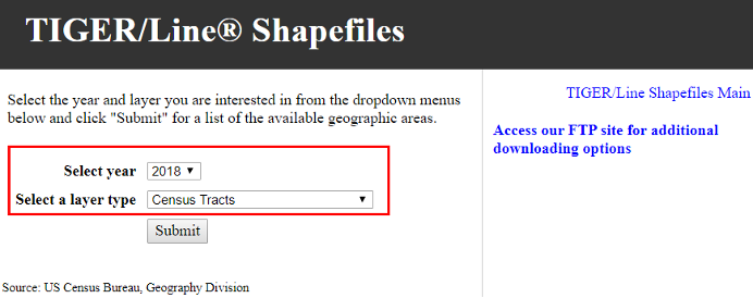
Go to this website. Note the available years.
Although the census tract geography is unlikely to have changed much from any given year, let’s select 2022 and click Web Interface option.
You will be presented with a number of geographies, including many we
mentioned in class, as well as several feature datasets (coastlines,
etc.). Under Select a layer type select Census Tracts and
click Submit.
Next, select ‘New York’ and click ‘Download’.
Save the zip file to your drive and unzip it. Open a new map in ArcGIS Pro and add this file.
Note the name designation of the file as well as the projection: Decimal Degrees. All census data is unprojected and utilizes a Geographic Coordinate System. Be sure to project it appropriately.
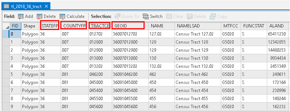
Open the attribute table and check out the attributes.
- We see column entitled GEOID, which appears to be a unique identifier for each tract.
- In the columns preceding it, we see the state identifier for New York (36), the county identifier (Tompkins is 109) and finally the individual tract identification.
- We can see that GEOID is simply a concatenation of these identifier variables. If we were examining smaller units (Blocks, Block groups), we would simply add on to this existing number.
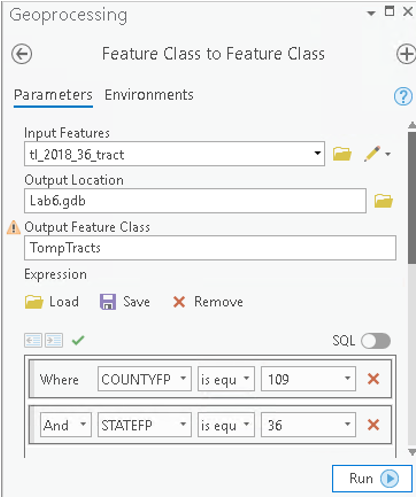
- Select the census tracts of Tompkins County and export to a new shapefile with an appropriate name, e.g., TompTracts.
At this point, you probably notice that this boundary shapefile does not come with the demographic data or other information you need, meaning you will have to separately download the information you need and join it to the shapefile.
Joining attribute information to boundary files
Now that we have our boundary file, we will need attribute table storing demographics or other information that can be joined to the boundary file.
There are couple popular site for downloading census or statistical data for a U.S study. They are the U.S census website (Go to https://www.census.gov/ in your browser. Or directly go to https://data.census.gov/cedsci/ if you already know what you are looking for by going to “Advanced Search”. ), social explorer, and IPUMS.
For this lab, we will specifically teach you how to download data from IPUMS and social explorer
Downloading data from IPUMS
Note: all the data has been downloaded for you in the lab data module: census_data_prep_manage_r.zip. You can review and practice the process but you can directly use the data from the folder to finish your tasks.
Go to the National Historical Geographical Information System (NHGIS) data website.
Click on the Login link in the upper right and follow the instructions to create an account. Back on the homepage, click on the Get Data link beside Start Here. Set the Filters as follows by choosing the selection, and then clicking Submit:
- Geographic Levels = county
- Years = 2020
- Topics:
- POPULATION General = Total Population
- Education = Educational Attainment
- Income = Personal Income
- Make sure to set “OR” as the Boolean value for topics - Datasets: 2020 American Community Survey = 2016_2020_ACS5a
Under the source tables tab, select the
- (B01003)Total Population
- (B15003)Educational Attainment for the Population 25 Years and Over
- (B19313) Aggregate Income in the Past 12 Months.
Under the GIS files tab, select the 2020 County file with the basis of 2020 Tiger/Line +. Under the Data Cart window in the upper right, click continue.
Make sure that you have three tables and one GIS file to be downloaded, and then click continue again under the Data Chart in the upper right. Under Table File Structure, select Comma delimited (known as .csv, best for GIS). Check the box to Include additional descriptive header row (best for spreadsheets), and click submit.
A .csv file can be understood as a clean, small, quick version of excel sheets, which is compatible with most of programs, from txt editor, Excel, Stata, ArcGIS, QGIS, to programming language such as Python and R, etc. csv file does not save format information (font, font size, bold/italic stytles, text color, graphs generated from excel, or the multiple sheets). That said, no matter how well you format the csv in Excel, generating beautiful tables, bar charts, multiple sheets, once saved as a csv, you only get the pure text/numeric content of the only FIRST Sheet.
After a bit, refresh the browser to see if the data is ready. Alternatively, check your email for a data link. Download the combined data table and the GIS County borders layers.
Unzip all of the files into a “Raw_Data” folder that you create. Make sure to stay organized by putting the contents of each zip into a named folder (IMPORTANT!!!). You may notice that the shapefile is double zipped and needs to be extracted more than once.
Start a new Arcgis Pro project, explore the GIS layer just downloaded to determine the projection. What projection is the data in? What will be the projection for the project? (You are mapping the contiguous United States).
Once downloaded, open the data in Excel. What we will do next is cleaning the data furthermore and make it ready and available to join to a spatial feature data in ArcGIS Pro. This part will be demonstrated during the class.
In general, you will always need to clean data before performing table join in ArcGIS Pro. Excel will satisfy some basic data cleaning need if the dataset is not too large. But remember to learn use R or Python to clean data in the future. (R demo from Canvas, after you run the R script, the cleaned data file will be in the output folder for you to use.)
In general, we need to utilizing the codebook (seperate file within your data folder) of your data to:
- Delete all the columns that don’t have any data.
- Keep all the columns related to education attainment of an bachelor degree or higher.
- Delete all the Margins of Error columns.
- Rename columns properly.
- Keep the GIS Join, State, and County columns.
- Create a new column and name it TOTAL_EDU.
After editing, save the file to a new csv file to your output folder.
Remember, our core purpose is to prepare the data table so that it can be joined to the attribute table of the shapefile. In order to do that, you have to
(1) change the structure of your joining table so that it is in the same data structure as your attribute table in ArcGIS Pro, and
(2) prepare and find your unique identifier. In most cases, GEOID or FIPS code is the most ideal candidate, but you have to be ready to find other unique identifiers when they are not available.
Joining data
Now let’s go back to the Map and try to join the data we just downloaded and cleaned with existing shapefile we have prepared.
- Add your excel table: cleaned_data.csv (note: you will need to click twice when an excel workbook is comprised of multiple sheets). Be sure it is closed out in excel!
- Open both attribute tables to make sure we know which variable we will use as our unique identifier. In this case, GISJOIN.
- Also note that both identifiers are in text format which enables us to join they directly. (As long as the format is match, it doesn’t matter what format it is! Can be both long, double, or text.)
- Close both attribute tables. Right click on our boundary file.
Select
Joins and Relatesand selectAdd Join. - For the join option, leave the default, and hit Run.
Open the attribute table for our boundary files. If you scroll over, the last column will be that joined from the excel sheet. After you joined, you must export the joined shapefile in order to permanently save your join.
- Map 6: Now create a quantitative bivariate map choropleth map depicting the income per capita and density of population with high education for only U.S continental. Before generate the map, you need to calculate a couple new fields within ArcGIS. Choose an appropriate color scheme, number of classification and classification method. Include all the elements for a proper layouts. (10 points)
Write a short answer describing the spatial relationship between the two variables based on the map. Also write your steps of choosing the appropriate classification method. (10 point)
You can also see this short video example to better understand the essence of table join in ArcGIS Pro!!
If you fail to join two datasets (it happens a lot!), you have to make sure the identifiers in two tables have the same format. Many failures to join the spatial boundary file with the associated attribute table are due to inconsistencies in data formats between the unique identifiers.
Note: another option to download the joined spatial data is through ArcGIS online Portal: From ArcGIS—>Add Data—>Online Portal—>ESRI Living Atlas, you can find the census data (linked geometries and tables).
Downloading data from Social Explorer
It is always good to have an great alternative data source. A number of private vendors have been established to make the process of accessing, managing, and interpreting census data easier. While Cornell has a license agreement for one of them (Social Explorer), many local governments, public agencies, community groups, Non-profits, and private firms may not, so it is important to understand how to access census data from different sources.
Here is an example showing you how to download from Social Explorer the same Census dataset we just downloaded from the Census Bureau website.
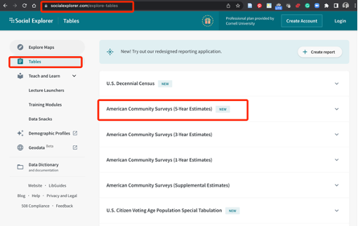
- Go to Tables —> American Community Surveys (5-year Estimates)
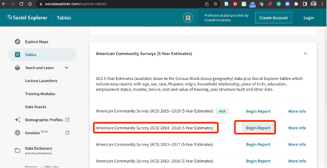
- ACS 2016-2020 (5-year Estimates), click Begin Report
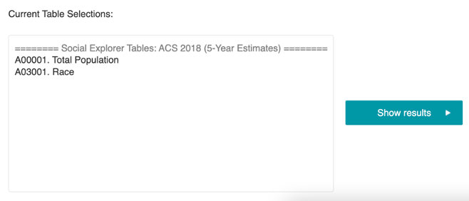
- In the selection page, choose “Census Tract” for “geographic type”, “New York” for “State”, “Tompkins County New York” for “County”, and “All census tracts in Tompkins County, New York” for “Select one or more geographic areas” and click “add”
- Click “Show Results”
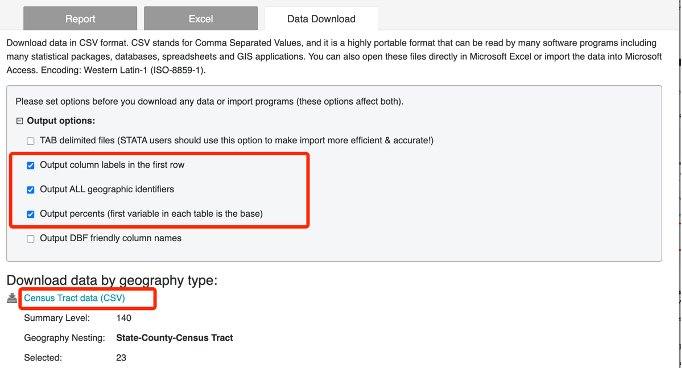
- Click Data Download
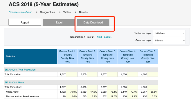
- Download the csv after checking these three options:
- Output column labels in the first row
- Output ALL geographic identifiers
- Out percentage (first variable in each table is the base)
The following instructions will lead you through using Social Explorer to export a dataset. Please learn how to access and download data from Social Explorer by yourself if you need more instructions: Guide.
Map 7: Use Social explorer to create a Total Population Change Percentage 2010 to 2020 map using census tracts and decennial census for your interested study area (if you don’t have one, you can just use Tompkins County).
- Clearly describe the data source you used in your map note (ACS or Decennial census? Which year?)
- Provide some interpretations of the map in the short answer.
To create this thematic map, you are required to login to Social Explorer using Cornell email and password. You need to download the 2020 population from the decennial census from Social Explorer. Open the table and browse to the last column, you will find the percentage change of population (2010-2020) for each census tract has been calculated for you!
Also downloading the 2020 Census boundary shapefile form either US Census Bureau website in the previous section or IPUMS.
- Make sure you download the boundary files (2020) to match the 2020 decennial census data.
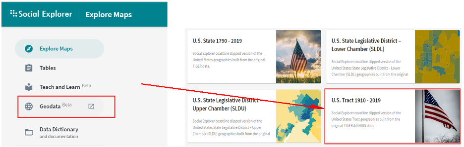
- The census tract boundary from social explorer (click “Geodata” from the menu bar and then browse to “U.S. Tract 1910-2019”), which stores all the historical boundaries at the census tract level, only update to 2019.
- You have to download the entire country and use “Select by attribute” in ArcGIS Pro to select your target area.
- For this exercise, please use the Geo_FIPS/Geo_GEOID as the unique identifier to finish the table join!
Now it’s your turn!!!
There are total 7 Maps for this assignment. (110 points)
Note from now on, be sure to include data source, data classification methods, projection information as part of the notes (inserted text) on each map layout!
And remember to start a new map session for different maps.
Map 1: (10 points)
Create a layout of normalized African American population (2000) for Tompkins County with a classification of your choice at the Census Tract level.
Map 2: (10 points)
Create a layout of normalized African American population (2000) for Tompkins County with a classification of your choice at the Block Group level.
Map 3: (10 points)
Create a layout of normalized African American population (2000) for Tompkins County with a classification of your choice at the Block level.
Question #1: (10 points)
Discuss how differences in the unit of analysis affects spatial patterns (i.e., the Modifiable Areal Unit Problem (MAUP)). (10 points)
Map 4: (10 points)
Create a layout of African American population (2000) per 1000 for Tompkins County with a classification of your choosing at the Census Tract level. Note that the African American population (2000) per 1000 should be shown in whole number in the legend.
Map 5: (10 points)
Depicting only those census tracts with a majority (over 50%) of renter-occupied housing units. Include a context map as well. Make sure that each selected tract is labeled with its Tract_ID value.
Map 6: (20 points)
Now create a quantitative bivariate map choropleth map depicting the **income per capita and density of population with high education for only U.S continental. Before generate the map, you need to calculate a couple new fields within ArcGIS. Choose an appropriate color scheme, number of classification and classification method. Include all the elements for a proper layouts. (10 points)
Write a short answer describing the spatial relationship between the two variables based on the map. Also write your steps of choosing the appropriate classification method.(10 point)
Map 7: (20 points)
Use Social explorer to create a Total Population Change Percentage 2010 to 2020 map using census tracts and decennial census for your interested study area (if you don’t have one, you can just use Tompkins County).
- Clearly describe the data source you used in your map note (ACS or Decennial census? Which year?)
- Provide some interpretations of the map in the word document.
Question #2: (10 points)
Please include a discussion of the differences between the 5-year and 1-year ACS estimates, described here: https://www.census.gov/programs-surveys/acs/guidance/estimates.html.
The END