Lab 4: Geoprocessing
Xiaozhong Sun
2023-05-07
Due Date: Lab_4 Due: Feb 22
Instructor: Xiaozhong Sun (xs243@cornell.edu)
Lab TAs: Ishan Keskar [iuk3@cornell.edu], Aditi Parihar [ap973@cornell.edu]
Location: Sibley 305, Barclay Gibbs Jones Computer Lab
Total Points: 110
Goals for this lab
In today’s lab, you will practice Geoprocessing tools in ArcGIS Pro, which includes:
- Dissolve features within a layer based on an attribute
- Clip one layer based on another polygon layer
- Intersect two layers
- Union two layers
- Merge two layers together
- Buffer features by a certain distance
- Use spatial join
After today’s lab, you will be able to choose the right and commonly used Geoprocessing tools to prepare spatial data for future analysis.
Know your data
For today’s lab, we will use
- Municipal Boundaries in Tompkins County
- Tompkins County Traffic Analysis Zones 2010
- Watersheds in Tompkins County
- Agricultural Districts for Tompkins County
- Tax Parcels in the Town of Danby as of 2014
- Landmark Buildings in Tompkins County
- Roads in Tompkins County
- East and West Hydrography for the Ithaca.
Preparation for Geoprocessing: some key points to note
Before doing any analysis functions in ArcGIS, such as Geoprocessing, you should make sure that all the data layers you will be using are in the same map projection/coordinate system, and that the data frame is also in that coordinate system (Apply what you have learned in lab_3). If you don’t do this, you’ll either get errors, or it will appear to run, but nothing will happen. For the purposes of this lab, all data is already in the same projection/coordinate system.
When using some of the spatial overlay tools, ArcGIS DOES NOT recalculate area, length, or perimeter, or any of the other attributes in the new shape file that results. (The attribute table won’t automatically update these parameters.)
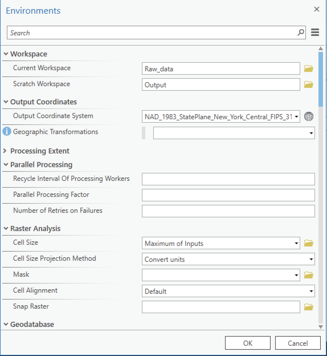
Before we begin, we firstly change the environmental settings that allow you to set up the default input/output workspace. This should become one of your routines for doing any spatial analysis in the future!
- Within the home folder stored everthing about lab_4, create an “Raw Data” folder that saves the Lab 4 data downloaded from Canvas, and an “Output” folder which you will save the outputs from running tools.
- After create a new lab_4 project file within your home folder. You
can specify Geoprocessing environment settings for your project using
the
Environmentswindow. These settings are saved with your project and will be automatically used by all tools that honor the environments. Open this window by clickingEnvironmentson theAnalysisribbon tab
- Under the
Workspacetab, set theCurrent workspaceas the “Raw Data” folder andScratch Workspaceas the ‘Output’ folder you created. Hit OK. Next time, when you select input features, ArcGIS will automatically navigate you to the current workspace by default, while the output layers you created will be stored into the scratch workspace. - Since we are working with data in New York State, you can also set
the
Output Coordinatesto StatePlane for this specific case and all your output features will be automatically projected.
Dissolving Features within a Layer based on an attribute
A dissolve creates a new layer in which all features that have the same value for a specified attribute become a single feature.
In this example, you will perform spatial analysis on the traffic analysis zones (TAZ) in Tompkins County. There are 365 individual TAZs in the county, but these TAZs only consist of 6 potential types. Let’s say you want to create a new data set that groups all the TAZs (i.e., feature) of a particular type (i.e., attribute) together, so that all the TAZs of a particular type are combined as a single feature. It would be useful to use the Dissolve feature to do so.
Note: Since the upgrade of ArcGIS Pro, it is equipped with more computational power, a new sets of pairwise overlay tools are now available. The pairwise overlay tools (Pairwise Buffer, Pairwise Clip, Pairwise Dissolve, Pairwise Erase, Pairwise Integrate, and Pairwise Intersect) are designed to maximize performance and accuracy of analysis during the processing of very large and complex datasets on a single desktop. The difference between them can be minor. If you want to know the detailed comparison between them, check this Blog.
Using ArcGIS online, add the following shapefiles to ArcMap: Search for Tompkins County Traffic Analysis Zones and add TAZ2010: A polygon of traffic analysis zones in Tompkins County. Note that the TAZ contains socio-economic data as well as information about employment density, etc. Also note that they are based on census block boundaries – we will be discussing census data aggregation more later.
Browse to the lab_4 data folder and add TCmunis - A polygon of the municipal boundaries in Tompkins County.
Dissolving Features Steps:
- Open the attribute table for TAZ2010 and take a look at the variable AREA_TYPE – this aggregates each TAZ according to whether it is rural, suburban, urban, etc. Symbolize TAZ2010 according to category of AREA_TYPE, so that there is a visual distinction between each type. Overlay the municipal boundaries so that the TAZs are revealed beneath them.
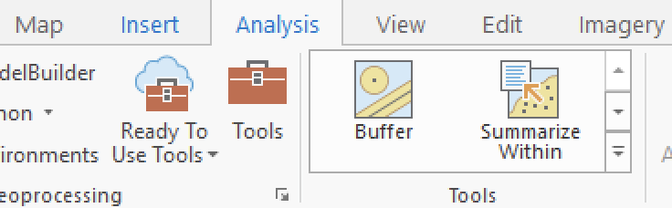
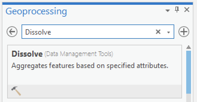
- Under the
Analysistab, underGeoprocessinggroup, ClickTools, in the search window, just typeDissolveand open it. You can also access a lot of often used tools in theToolsgroup drop-down list.
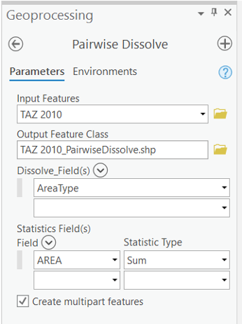
- In the dialogue box: (1) select TAZ2010 as the input Feature, (2) it
should automatically specify the output name (e.g.,
TAZ2010_dissolve, or TAZ_PairwiseDissolve) and location for saving the
file (i.e., your output folder), (3) Under
Dissolve_Field(s)select AREA_TYPE - this is the attribute on which you want to dissolve. In order to obtain a total area for each TAZ type, select AREA inField. Then underStatistic Type, selectSUM. This will create a column with the new areas. Click Run.
- Review and compare the new data and the original one: The new shapefile, TAZ2010_ dissolve, is automatically inserted into the Contents Pane. Modify the symbology of the new layer according to AREA_TYPE, as in Step 1. Note the difference between the dissolved and original TAZ dataset. Compare the attribute tables of these two datasets. Since the boundaries between polygons of the same AREA_TYPE value has been joined together, a lot of the attribute information has been dropped. This is a common (often undesirable) result when dissolving features. However, note that we now have a field entitled ‘SUM_AREA’ which is the aggregation of all the TAZs within that particular area type.
- With the attribute table for TAZ2010_Dissolve open, go to the
menuon the top right and selectExport.
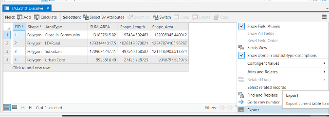
Export the dbf. table (It is important to assign it a different name under Output folder than TAZ2010_dissolve.dbf since a file of this name already exists, otherwise the process cannot be done.) into your own folder.
- Open your exported .dbf in Excel (Note: ArcGIS creates several files when exporting the attribute table including a dbase table and an xml file. Be sure to open the dbase table, not the xml file!!). Also note if you fail in opening the .dbf, you can firstly open an empty Excel and drag the .dbf into it.
- Calculate a new column with the Percentage of total area for each TAZ type in Excel. You can also edit the table and data in Excel to make it look more presentable. Also, be aware that two significant digits is sufficient for the value.
Map 1:
Create a map layout that shows the dissolved traffic analysis zones across Tompkins County, with the municipal boundaries overlaid. Provide a summary table that includes the Name of Area Type and the percent of the total of each type on the map layout with all necessary elements.
Note: The easiest way to insert a table into a Map layout is to copy and paste the table directly from the Excel. Save your project and start a new map session.
Clipping one layer based on another
Clipping trims features in one layer at the boundaries of features in another layer and is a very important data preparation tool. You should note that after clipping the attribute information is not combined. Clipping is an important feature in performing spatial analysis, because many times, features do not adhere to certain boundaries, man-made or otherwise.
For instance, each of the six watersheds that are found in the City of Ithaca extends beyond the city limits. If you wanted to quickly measure the area of the portions of each watershed that lies within the city boundary, clipping the watersheds layer to the city boundary would be a useful function.
Create a new Map (on the insert tab) and name it ‘Clip.’ Add the following shapefiles from our local folder: watersheds.shp – most recent polygon theme of watersheds in Tompkins County (Note: this is a shapefile of watershed already clipped to Tompkins County boundaries); TCmunis - A polygon theme of the municipal boundaries in Tompkins County. Since we already added this to your project, simply copy and paste from the original data frame to the new map.
- Open the attribute table for watersheds.shp, examine the information and symbolize according to the category of WATERSHED (without “S”), so that there is a visual distinction between each watershed. Overlay the municipal boundaries to reveal the boundaries of each watershed.
- Prepare a shapefile to serve as the “Clip” layer: Based on the TCmunis layer, create and export a City of Ithaca (not town of Ithaca) boundary shapefile (renamed of course! Note: You already know how to do this from previous labs. After export,add your new City of Ithaca boundary.
- For the original TCmunis layer, you can now clear the selection and turn off the layer. TCmunis has served its purpose
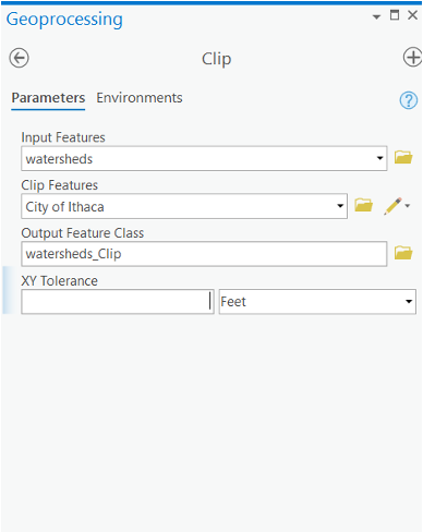
- Under the
Analysistab, select theClip(As above, search for it). We will now clip watersheds to fit the city of Ithaca boundaries. In this case we are not interested in the attribute information of the City of Ithaca, but only its geographic extent. Clipping is often considered more of a data preparation tool. - In the dialogue box: (1) In the
Input Featuresdrop-down list, click watersheds as the input layer, (2) In theClip Featuresdrop-down list, click city of Ithaca which was created in Step 2 as the polygon clip layer, and (3) specify a file name that is clear, simple and understandable, and location to save the new file. Click Run.
NOTE: Open the attribute tables for both the original and clipped watershed layers. You can toggle back and forth between watersheds and watershed_clip using the tabs. From the original layer of 15 different watersheds, only six watersheds were selected that are partially within the City. Compare the Area values for a specific watershed (i.e., West Cayuga Lakeshore) in both tables. Notice that even though the areas have changed dramatically, the attribute values have not been modified. That is, the AREA of the clipped features still represents the area of the entire watershed. This is because the clip function merely functions as a ‘cookie cutter’ and does not affect the attribute information at all. To rectify this, we need to update the areas values by editing the table and calculating some new values.
Now let’s update measures of watershed area within the City of Ithaca:
- Clear the
Selection, and with the attribute table for the clipped watersheds open, selectAdd Field
- Make sure the current layer is set to Watershed_clip.
- Enter the name ‘New_area’. ‘Double’ for the Data type (this refers to the types of field data allowed in each cell; see here for a description of the various field data types) and ‘Numeric’ for the Number format (limit the rounding to 2 decimal places).
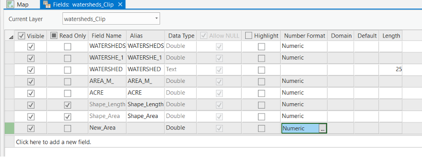
- Click Save

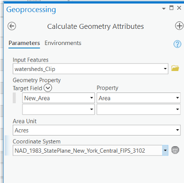
Changesgroup). There should now be a new column called ‘New Area’ that is filled with Null (or zero) values. - In the attribute table, right click ‘New_area’, select
Calculate Geometry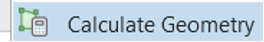
Target fieldto New_area, thePropertyto Area, thearea unitsto Acres, and theCoordinate systemto the Current map (NY State Plane central). Click Run.
- Now export your new attribute table, open it in Excel to create a table with only WATERSHED and New_acres (Follow similar steps as Map 1).
Map 2:
Create a map layout that shows the watersheds in the City of Ithaca, clipped to the city boundary. Provide a summary table that includes the watershed name, total number of acres of each watershed within the city, and the percentage somewhere in the layout (you should calculate the % area of each watershed in Excel). See earlier instructions on including a table in layout.
Intersecting features from two layers
In this exercise, you will use the intersect functionality of ArcGIS to identify all tax parcels located within an Agricultural District in the Town of Danby. When intersecting features from 2 layers, we identify just those features that spatially overlap from both layers. The output file contains attributes from both input layers.
Keep in mind that the Intersection feature differs from the Clip function in that the field information from BOTH the input and overlay layer are retained in the output feature, whereas in the Clip function only attributes of the input feature are retained.
Create a new Map and name it “Intersect”.
Add the following shapefiles to ArcMap: TCmunis - A polygon theme of the municipal boundaries in Tompkins County; agdist.shp - A polygon feature of agricultural districts for Tompkins County; dparcl2014 - A polygon layer of tax parcels in the Town of Danby as of 2014.
Steps:
- Based on TCmunis, create a shapefile of Town of Danby boundaries. Once you have added the newly created Town of Danby boundary file to ArcGIS as a new layer, Remove TCmunis.shp from the Contents Pane.
- Go to the
Analysistab and selectIntersect.
- In the dialogue box: In the
Input Featuresdrop-down list, click agdist and daprcl2014 as the input layers. In theOutput FeatureClass, specify a file name, parcel_agdist, and save the new file to your folder. Click Run.
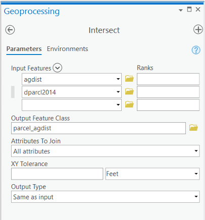
- Review the output shapefile. The Intersect function selected only those Danby tax parcels that are located within the boundary of Agricultural District 1 and Agricultural District 2. Open the attribute table of this layer, parcel_agdist, and notice that the table has a DISTRICT field with values of 1 or 2 from the agdist.shp, as well as parcel information from the daprcl2014 polygon layer.
- Right click on the column header for the “MUNICIP” field and click ‘Sort Ascending’. Scroll down and note that there are several parcels that belong to the Town of Ithaca, Town of Newfield, Town of Dryden and Town of Caroline (if you zoom in, you will see that these are by and large sliver polygons left over from the intersect, these features are left-overs of the agriculture district layer.). Select only the Town of Danby’s tax parcels and export the selected parcels to your folder, danby_parcel_ag. Remember that most Geoprocessing functions do not affect the attribute information at all. To rectify this, we need to create a new field and calculate the new areas (you should know how to do this form the previous step). Calculate the new parcel area as acres.
Map 3:
Create a map layout depicting Tax Parcels in Danby that are located within a designated Agricultural District. Symbolize this layer according to District number. Include Town of Danby boundary. Provide a table that includes: the number of tax parcels and total acreage in both Agricultural District 1 and Agricultural District 2 in the Town of Danby.
Save your ArcGIS project.
Buffering Features
A buffer is a region of a specified distance that surrounds certain features and can be uniform or variable in width; buffers can be effective for performing analysis that examines the proximity of one feature to another.
For this exercise, you will apply a uniform buffer around all fire department facilities to determine the extent of the service area, and to identify the areas which fall outside of the existing Service Areas.
Create a new Map, and name it ‘Buffer’. Add the following shapefiles to Arc Map: TCmunis - A polygon theme of the municipal boundaries in Tompkins County; landmark.shp - A point feature of landmark buildings in Tompkins County.
Steps:
- Open the attribute table for the landmark.shp layer. This lists public institutions and facilities in Tompkins County. If you scroll, you will see that the attributes information includes street addresses – this data has been geocoded – something we will be exploring later on.
- Based on the “SERV_TYPE” field, select out all fire departments and create a new data layer to be added to your project (be sure you rename your layer!).
- Go to the
Analysistab and selectBuffer.
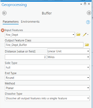
- In the dialogue box: (1) in the
Input Featuresdrop-down list, select your Fire Departments shapefile, as the layer to buffer, (2) in theOutput Feature Class, specify a file name, Fire_dept_Buffer, and location to save the new file, (3) set the buffer linear units to Miles, and specify the Buffer Distance as 3 miles (Note that we could also buffer the feature based on a particular attribute field) and (4) select Dissolve Type as “ALL” (this will ensure that if 2 buffer polygons overlap, they will be merged into a single polygon). Click Run.
- Now perform an additional spatial analysis by adding a shapefile of Tompkins County roads (you can import a road layer from ArcGIS Online Portal or All Portals) and clipping the roads layer to match the spatial extent of the buffer layer.
Map 4:
Create a map layout that includes fire stations and all roads that fall within 3 miles. In addition, you should include your buffer polygon and municipal boundaries. Save your project. We will continue this analysis in the next section.
Unioning Two Layers
A union is a topological overlay of two polygon datasets that preserves both the spatial extent and the attribute information of both input layers. Thus, Union is similar to intersect in that both retain the attribute information of both. Where they differ is in the spatial extent (think of an ‘and’ verses an ‘or’ statement). In this example, you will Union the areas that fall outside the service areas of the Fire Department buffer layer with the corresponding area of municipalities in Tompkins County.
Create a new Map entitled ‘Union’, the data you need are TCmunis - A polygon layer of the municipal boundaries in Tompkins County. The buffer output file, fire_dept_Buffer, created in part 4.
- Go to the
Analysisribbon and selectUnion.
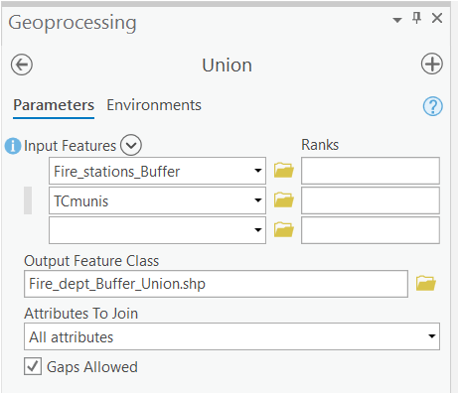
- In dialogue box: (1) in the
Input Featuresdrop-down list, Select the three mile Buffer of Fire Stations (from part 4), Fire_dept_Buffer, and munibnds.shp as the input files and (2) in theOutput Feature Class, specify a file name, Fire_dept_Buffer_Union. Click OK.
The new layer, Fire_dept_Buffer_Union, is added to the table of contents. Remove the 3-mile buffer layer, Fire_dept_Buffer, from the Content Pane. Position the Fire Departments layer at the very top of the Content Pane, and TCmunis.shp at the very bottom.
Examine the output of the Union: Open the attribute table for the Unioned layer, and notice the field titled: FID_ Fire_ d. Each record has a value of either “-1” or “1”. Those records with a value of “1” fall within the 3-mile service area, and those with a value of “-1” fall outside the 3-mile buffer within Tompkins County. We will now create a new shapefile based on the Unioned layer containing only areas outside the service buffer zones.
While we could do this as we did earlier, by selecting attributes and exporting a new layer, we will try a different approach this time.
- Open the attribute table for the shapefile, Fire_dept_Buffer_Union.
- From the Selection Options, choose
Select by Attributes
- Hit “Delete” button on the keyboard or the “Delete” button in the
attribute table. The remaining records are all the features that fall
outside of the 3-mile service areas.
- Go to the
Edittab, and clickSave
Notice: This type of buffer analysis is very simplified and does not take into account road networks or barriers. Rural areas have fewer roads and therefore it may take longer to reach a home within a 3- mile radius; thus, the radius of service areas in rural areas would likely be smaller than it would for a fire station responding to a call in the urban core. This type of buffer analysis also doesn’t take into account certain physical barriers, such as Cayuga Lake, which obviously impacts the real extent of a station’s service area. The Network Analyst Extension can be used to identify service areas in a more sophisticated way – we will explore network analyst in a later lab.
Map 5:
Create a map layout that shows Fire Stations (labeled with the Fire Station name), the Tompkins County municipal boundaries, and the Gaps (area outside the buffer of service region) in the fire service area. Save your project.
Merging Layers
Use Merge when you want to combine two or more adjacent layers (that share a common border) into one large layer that contains all their features.
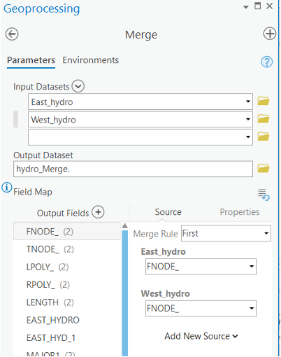
Create a new Map entitled ‘Merge’ and add the following shapefiles from the folder: East_hydro — A shapefile depicting hydrography for the Ithaca East USGS 7.5’ Quadrangle; West_hydro — A shapefile depicting hydrography for the Ithaca West USGS 7.5’ Quadrangle.
Note: Both of these shapefiles are originally based on coverage file formats (an earlier file format no longer used), hence the boundaries of the shapefile are shown as part of the shapefile.
Steps:
- Go to the
Analysistab and selectMerge.
- In the dialogue box: in the Input Features drop-down list, select both the East_hydro layer and the West_hydro layer as the layers to merge. Specify the name and location of the output shapefile in your personal lab_4 folder, hydro_Merge. Click Run.
Map 6:
Create a map layout that depicts your newly merged hydrology layer clipped to the City of Ithaca boundaries.
Spatial Join
Create a new Map entitled “Spatial Join”. A major difference between the Spatial Join and the other Overlay tools is that the Spatial Join does not alter the original geography in any way. It simply joins the attribute tables of two layers together based on common spatial locations. In that way it is similar to a table join (based on a common attribute field value) – we will explore this in a later lab.
The other Overlay tools will result in altered geography – for example, if you perform an Intersect between town boundaries and water bodies, the result will be a water bodies layer where water polygons are split at town boundaries instead of crossing them. This would then allow you to calculate the total surface area of water bodies per town.
For this section, add the following shapefiles to your new Map: TCmunis- A polygon layer of the municipal boundaries in Tompkins County; landmark.shp - A point layer of landmark buildings in Tompkins County.
We are already familiar with these files, so no need to examine the attribute table.
- Go to the
Analysisribbon and selectSpatial Join.
- Under
Target Featuresadd landmark. - Under
Join Featuresadd the municipal boundaries. - By specifying this order (order matters), we are instructing ArcGIS to join municipal boundaries to landmarks based on spatial location. This implies that the attributes of municipal boundaries will be joined to the attributes of landmarks where they overlap.
- Set your Output feature class to your working drive and save the file as something you will recognize.
- Under
Join Operationnote your options:One to manyorOne to one.
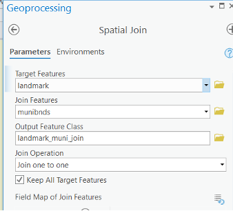
A) Try both the “One to many’ and ‘One to one’ option.
- Does it matter in this instance if you chose ‘one to many’ or ‘one to one’?
- Why or why not?
Open the attribute table of your new spatially joined landmarks layer. You will see each landmark has accompanying information related to the municipality without altered the original geography.
Now run a second spatial join, this time with municipal boundaries as the target layer and landmarks as the join feature. (Change the order)
B) Try both the ‘one to many’ and ‘one to one’ option.
- Does it matter in this instance if you chose ‘one to many’ or ‘one to one’?
- Why or why not?
Answer the Questions:
Note that the ‘one to many’ join contains an attribute entitled ‘Join_Count’. What does this reflect? There is no map layout required, but you must answer the questions (including A and B) highlighted above.
Now it’s your turn!!!
Part 1. (Total 80 points)
- Finish Map layout for Maps 1 – 6. (60 points, 10 points each)
- For Maps 1-3, please also provide the summary tables (5 points each)
- Written Answers to Part 7. (5 points)
Part 2. (Total 30 points)
1.Complete the following overlay analysis and include a short write up of the steps you followed to complete the task (15 points)
Identify all areas within the Fall Creek watershed that lie within 500 feet of streams and lie within an Agricultural District. Use the following input shapefiles:
- Watersheds.shp - polygon of watersheds in Tompkins County (Note: this is a shapefile of watershed already clipped to Tompkins County boundaries);
- Hydrology: A shapefile of streams within Tompkins County;
- agdist.shp - A polygon of agricultural districts in Tompkins County.
2.Create a map layout of the results. (10 points)
Please reference data (i.e., Municipal boundaries), or anything else you think may be useful in helping the reader interpret the map.
3.Answer the Question: What percentage of Fall Creek watershed meet these criteria? This will require you to recalculate areas (5 points).
The END