Lab 5: Georeferencing and Onscreen Digitizing/Editing
Xiaozhong Sun
2023-05-07
Due Date: Mar 3th
Instructor: Xiaozhong Sun (xs243@cornell.edu)
Lab TAs: Ishan Keskar [iuk3@cornell.edu], Aditi Parihar [ap973@cornell.edu]
Location: Sibley 305, Barclay Gibbs Jones Computer Lab
Total Points: 100
Goals for this lab
- Understand what is georeferencing
- Create and edit shapefiles in ArcMap
Know your data
For today’s lab, we will use a couple image data/raster data, a coastline shapefile, a CAD image file, Tompkins County roads (roadcl.shp) and building footprints (buildings.shp).
Georeferencing is a process of making image data spatial. For example, an aerial image of Sibley Hall contains information about the footprint of the building in relation to the Arts Quad and other surrounding buildings, but without contextual information about these features, it does not reveal the location.
Georeferencing ties specific points on the image to specific points on the Earth’s surface. Remember from the previous lab work on projections that unprojected data cannot be located geographically. Similarly, without reference points, image or raster data cannot be located on the Earth’s surface.
Georeferencing a Map Image
Raster data is commonly obtained by scanning maps or collecting aerial photographs and satellite images. Aerial photographs and satellite images require additional locational information delivered to ensure they align properly with other spatially referenced data. The process used to locate an image on the surface of the Earth, in other words, to a map coordinate system, is called georeferencing.
When you georeference your raster file, you define its location using map coordinates and a coordinate system. Georeferencing raster data allows it to be viewed, queried, and analyzed with other geographic data. In this exercise, you will apply this using a scanned US Geological Survey Map from 1894.
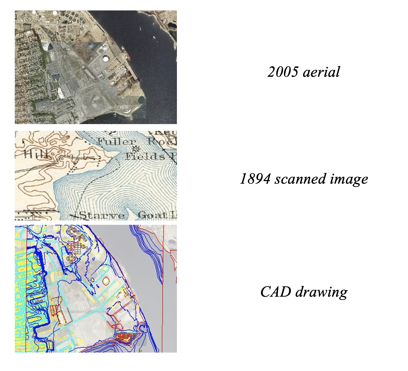
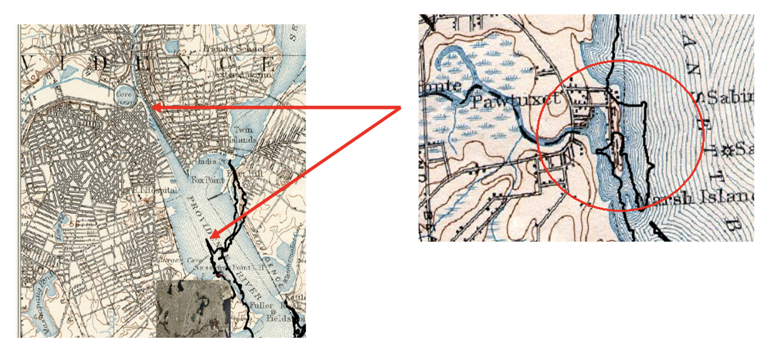
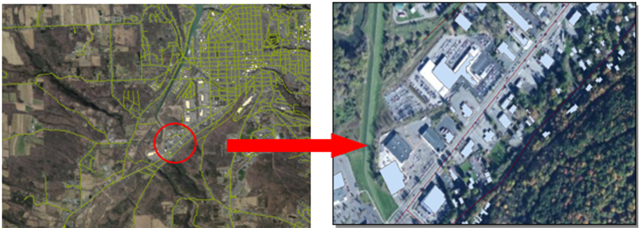
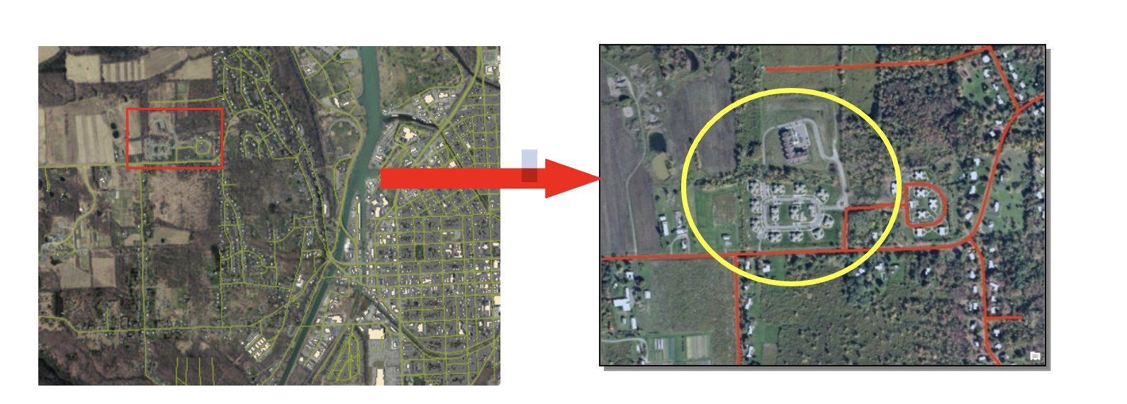
These images below of the same area come from a different of sources and are in different scales. Georeferencing will enable each to be layered accurately upon one another.
Georeferencing the 1894 Map
The goal of this exercise is to tie an aerial photograph (raster image) to coordinates representing their location on Earth. In other words, we want to ‘georeference’ our aerial imagery.
To do this, we have to use a reference data file of the same area.
This reference layer – called the “target” data within some GIS software – could be any format of referenced spatial data depicting the same features.
With the ubiquity of satellite data (Google Maps, Bing Maps, and on and on), this task has become easier.
The target data could also be a vector representation of the same features.
Getting started:
- First, copy the data from the course folder to your own folder.
- Now, create a new ArcGIS project and add Coastline.shp to the Map view.
- Open layer properties and note its projection – Rhode Island State Plane. This is the coastline for the state of Rhode Island. This will be our target data set.
- As mentioned above, our target data must have a projection. Check to see if the coastline has a projection. Note that the Map View has assumed these projection properties.
- Now add 3426.sid. this is a 2005 aerial image of
the site. Note: If you use the “add data”, just highlight the image file
name and press the “Add” button.
- If you double-click the filename, it will show you the contents of the file (three bands of the image) and ask you to choose a band.
- In some cases, you may want to choose only one band, but in this case, you want the full file.
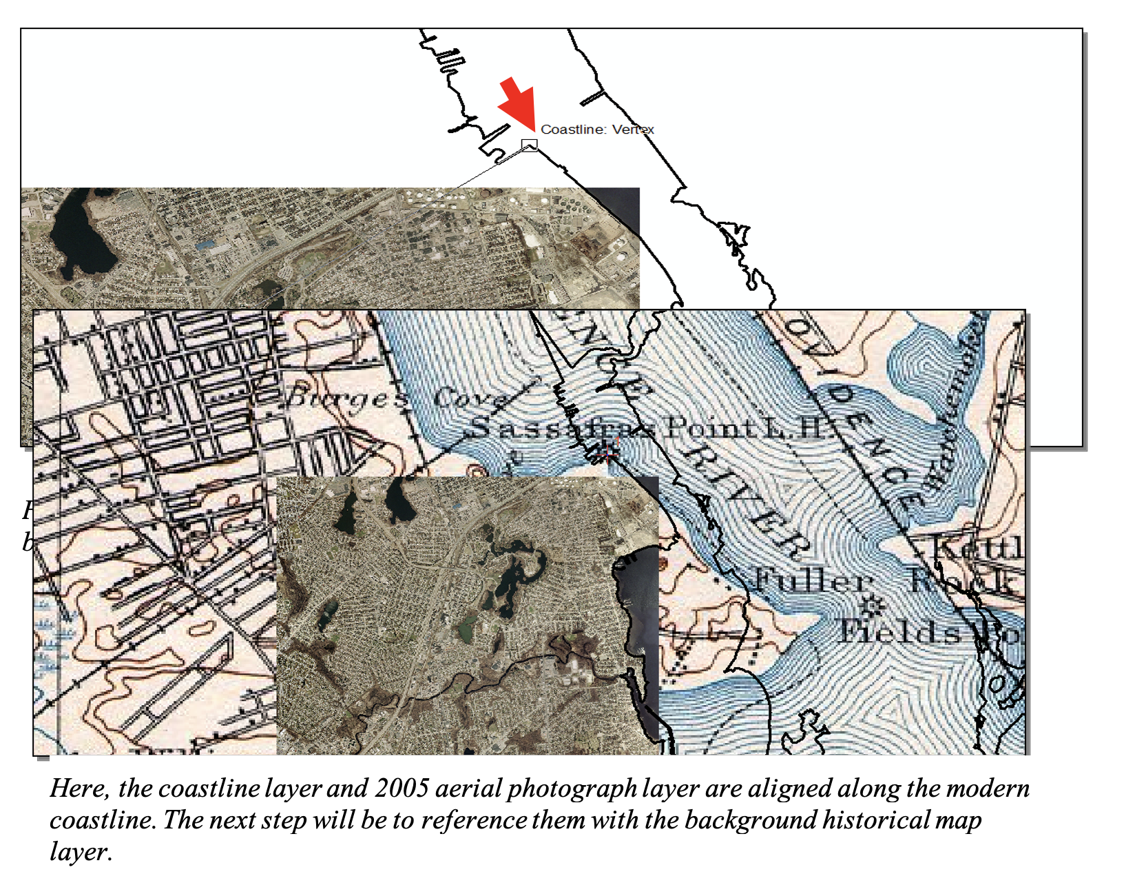
- Zoom in and you should see that the coastline and the aerial should line up.
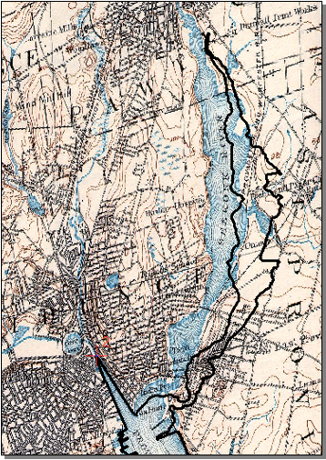
- Now add prov94sw.jpg, a scanned USGS map from 1894.
- It does not show up on top of the other data we’ve added.
- Find it by zooming to layer.
- Take a close look at the map image and note the shape of the coastline.
- For example, look at the shape of the Providence River as it flows out of Downtown Providence – almost in the center of the map.
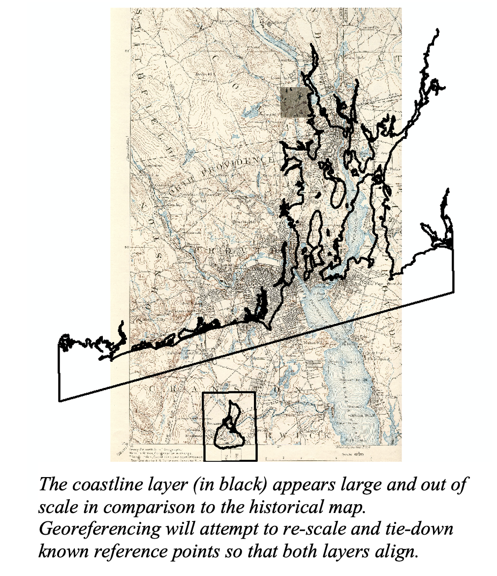
- Now zoom to your Coastline layer.
- It will help if you set the symbology for this layer to remove the opaque fill and make the outline thicker.
On the Imagery tab, click Georeference to
open the Georeference tab (you may need to click a raster
layer first to enable this function). The Georeference tab
contains all the tools you need to georeference your raster
datasets.
In the Contents pane, select the layer you want to georeferenced (prov94sw.jpg).
- Turn on
Auto Apply
- Choose
Fit to Display
We will set one point on the historical map, then we will set
a matching point at the same location on the coastline. On the
georeferencing toolbar you will see the
Add Control Pointsicon
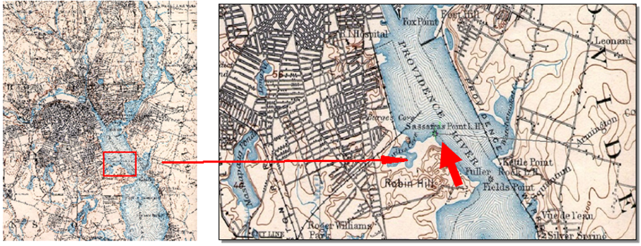
We will first locate a point on the historical map (“from point source”). What kind of point do we want? This is tricky, as the site has been altered since 1894, so we need to find a point that has remained the same. In fact, we will need to find several points to accurately georeferenced the image. In locating points, we will have to zoom in and out, pan, and turn layers on and off.
Sassafras point lighthouse is one such point – there has been minimal alteration to the landscape at this point. Add your first control point here. Notice that you get a green crosshair graphic, and a rubber band line that extends as you move your mouse. If you are not happy with your control point, press the Esc key to remove a link while you’re in the process of creating it.
Now we find the complimentary point on the coastline map to place the
other control point. Zoom out (the control point will remain active
while you do this). You can use the direction buttons in the keyboard to
move the extent to the corresponding point in the coastline layer. Now
zoom back in the modern-day location of the Sassafras point lighthouse
upriver and just outside of the range of the 2005 aerial photograph. You
will have to sequentially zoom and pan until you find your way around
(Be careful, at this point it is easy to get lost and forget where your
initial control point was.) If you are not happy with your control point
or a reference link, you can delete an unwanted link from the
Control Point Table
Place your second control point - Notice that it appears as a red
crosshair. We have now created our first control point “link.” Take a
look at the Control point table - we have successfully
added the first ground control point. Make sure that the
Auto Apply box in the Georeference tab is
checked. Notice how the layers adjust to better line up. A good start -
but it could still use some improvement (if you zoom out you will see
that the Providence River is still mismatched).
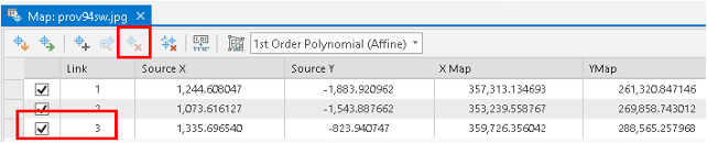
Add at least 2 other control points. Remember that your first point has to be on your source historical map, and the corresponding point (the second one) on the coastline map.
If you do the process in reverse, bad things happen. The minimum links we need are 3 (first-order polynomial transformation). (Note: often placing more control points does not necessarily produce a better result.) Because the historical map and coastline shapefile are somewhat more aligned than before, the process of finding similar points should be easier. One possibility is downtown Providence, where the river narrows considerably.
Notice the approximate location of each area on the different layers. Choosing a point in downtown providence will allow a better georeferenced to occur and allow for a better fit.
If you zoom out, you will notice that the historical map occupies a much smaller segment of the actual coastline shapefile – not an ideal situation when georeferencing. Let’s add a third point, away from the other 2 points. Further downstream, near ‘Pawtuxet’, we note a small peninsula that appears to have been already settled in 1894, as well as its modern-day incarnation nearby. Link the ends of the two peninsulas. You may get a warning message, read them and accept the warnings by clicking OK.
However, note that the 1894 map is now rather contorted as it tries to match all 3 link points. Moreover, if we pan back upstream, we see this:
Adding that 3rd link downstream appears to have increased the distortion upstream as ArcGIS tries to force these 2 coastlines to match. Perhaps 3 links are too many, or not suitable? Open your link table and remove that third link.
Note how the maps shift in response. Let’s try adding a third link upstream. Pan upstream to the settlement north of Providence (close to Hammond Pond). The Coastline layer ends where the river narrows as it goes around the bend. Link these 2 layers based on the narrowest point.
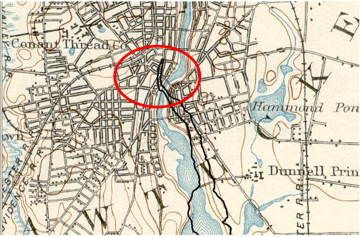
Once completed, zoom/pan around and check out your match. While we appear to have avoided similar distortions down river, it’s unclear whether or not this third link point adds much value. Check out the area where we made the first match point (this is also where the aerial photo has coverage). Regardless of how bad our match is, there is no way the discrepancy between coastlines here is only due to inconsistent data.
What could
explain the discrepancy between the 2 coastlines?
A note on the Control Point table: You can save your Control point
(link) table (a good idea if you want to come back later and improve
your registration) using the disk
icon
Map 1: Create a layout of the historical map and the Coastline (only include those areas in your layout that cover your match points). Discuss some reasons why they don’t line up more closely.What could explain the discrepancy between the 2 coastlines?
Georeferencing CAD files
Georeferencing a CAD dataset is very similar to georeferencing an image. However, you are only allowed two sets of control points for a CAD file links table. If you have more than one CAD layer in the map that derives from the same CAD file, you can use any one of the layers for the transformation; the transformation will apply to the entire CAD dataset.
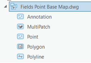
Open the Catalog Pane and navigate to the CAD file (in
.dwg format) called Fields Point Base Map.dwg. This is
a CAD drawing that includes coastlines as well as streets, contours, and
building footprints around the site. Note that it includes multiple
files; each of which corresponding to a unique spatial feature, e.g.,
Annotation, Point, Polyline, Polygon, etc. The polyline layer contains
the site information we are interested in. Drag this layer to the
contents pane. Zoom out and you will see that this layer needs
georeferencing. Note that you will georeference the CAD map to
the coastline layer.
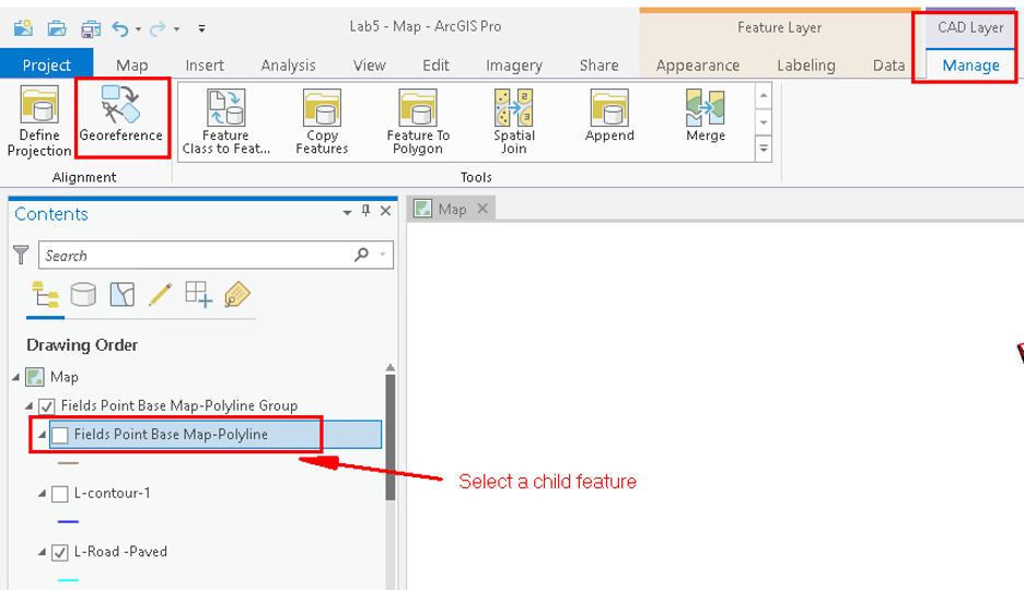
To do the georeference for a CAD layer, we need a
CAD layer tab. The CAD Layer tab is not
visible when a CAD group layer is selected, e.g., choosing the whole
polyline layer. To display the tab, select a child (sub) feature layer
in the CAD group layer and the CAD Layer tab will
automatically pop up in the ribbon. Georeferencing a single CAD feature
layer applies that transformation to the entire dataset. Once you have
georeferenced a CAD feature layer, you can add the other feature classes
of that dataset to the map, and they will be constrained by the same
control points.
Note: Georeferencing a CAD file is somewhat different – you first
need to add both of your control points (only 2 sets), and then hit
Apply. A point at the CAD and a corresponding point
on the coastline layer together means one set control point. So, you
should totally determine 4 points (two points per layer).
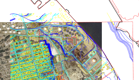
Map 2: Create a layout of your CAD file correctly georeferenced.Include Coastlines and the aerial photo as well. For your layout, please zoom in on the portion of the CAD drawing that includes roads, building footprints, etc. – do not include the full extent of the CAD drawing!
For this map layout, you don’t need to include a legend for the CAD layers. However, you need to write a short sentence in the note describing what you are georeferenced!
Save your ArcGIS Pro project – we will be returning to it later on.
On-screen Digitizing and Creating New Vector Data
In this section, we will utilize onscreen screen digitizing to edit and create shapefiles in ArcGIS Pro.
- Start a new Map project, add Tompkins County roads (roadcl.shp) and building footprints (buildings.shp) to the contents. In the Map tab, click “Basemap.” You will see a number of options. For now, add ‘Imagery’.
- Zoom over (hint: turn off base map while you are zooming will make processing much quicker) to the Route 13 corridor (just south of Walmart). You can also search location like we talked back in lab_1. Notice that there are several new buildings constructed since the original ‘buildings’ layer was created.
Creating a new shapefile
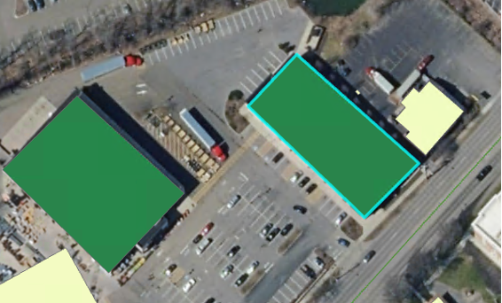
Instead of editing the ‘Buildings’ layer, let’s instead create a new shapefile of some of the building footprints not yet digitized.
- Go to
Catalog Pane(View->Catalog Pane). Right click on the folder you are using for this lab. Go toNewand thenShapefile.
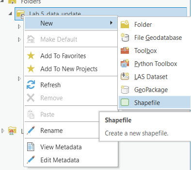
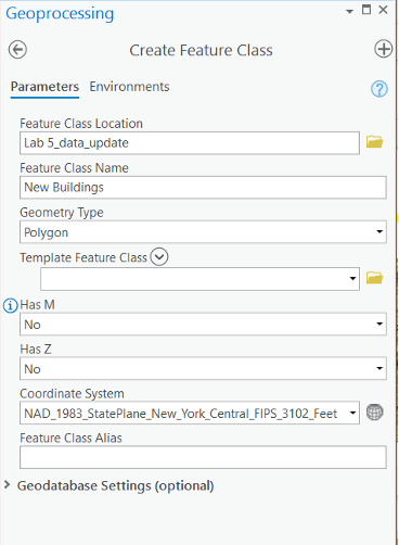
- For name use ‘New Buildings’. Change the Feature Type to “polygon.”
- Set the coordinate system to buildings (so that they are of the same coordinate: New York State Plane central. Click Run.
- Back in the Map View, the “New Buildings” should be added. It’s
empty, so nothing comes on the screen, but if you check the properties
of the layer, you will see that the projection information has been set.
So has the scale and map extent.
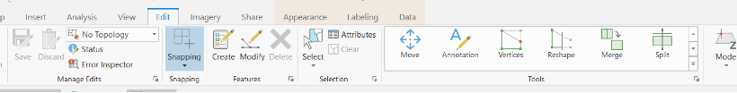
- Click on the
Edittab at the topic, and a number of tools will appear.
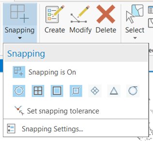
Setting the snapping options
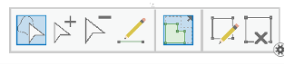
Open the snapping options (blue box indicates active). Hover over
each icon to see which option each represents. Click on the
Snapping Settings at the bottom of the snapping
drop-down.
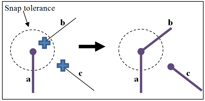
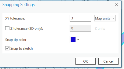
This should display a window that allows you to set the XY tolerance or snapping tolerance. The snapping tolerance is the minimum distance between two vertices at which they are considered to be identical. If the cursor gets within the tolerance of a vertex, the next mouse click will be snapped to that vertex.
Note that we can set to either pixels or Map units. It is typically best to set to the map units specified by the projection, and set a snap distance in map units. It ensures consistent precision at all scles. But may become difficult to work with when zoomed far in or far out from normal editing scale.
Set your XY tolerance to some number between 2 and 4 map units and click on OK. The end use specifies the data accuracy requirements, but if you set the snapping too small you end up with inefficient digitizing.
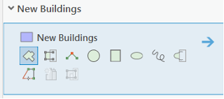
- Click the
Createtool
Create Features paneshould appear. Select ‘New Buildings’, as this is the shapefile we are interested in editing. - This opens up some additional tools for digitizing. Select the
Polygontool.
If you pan over the Map, cross hairs should become active. Outline
the new building. As you do so, notice a floating tool bar. If you make
a mistake, click
cancel

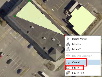
Try adding several other buildings. Note that we have not actually created any attribute information – we would need to separately edit the attribute table.
Adding Vertices to an Arc
Sometimes you will want to add vertices into a straight segment of an
already existing polygon, in order to improve the accuracy. Activate the
Modify tools with the icon found along the main Edit tools
ribbon
This will highlight a number of alignment and reshaping tools. If you
click the Edit vertices
tool
Experiment with adding and deleting vertices. Once added, you can
also move the vertex. To adding or deleting vertices, you need firstly
select a feature

Moving a Vertex
Sometimes you may want to move an existing vertex of a polygon.
Select the normal
tool
Once you’ve edited this boundary to your satisfaction commit your changes.
Commit the Changes
The changes you make are not committed until you save so. Go ahead
and commit the changes now
(finish)
Save your edits often. When finish adding new buildings, close the
modify panel and clear any selected features.
Digitizing Lines
If you have not yet done so, please add roadcl.shp and change the symbology so that it is visible against the aerial basemap. Pan over the West Hill and note that there is new housing and roads that have been constructed off of Mecklenburg Road (Route 79). We will edit the existing roadcl layer to reflect these changes.
- In the
Create Featuresbox, highlight the ‘roadcl’ layer. SelectLine. - Note that as you pan your cursor over the map, a little circle or square picks up the vertices of the road layer. Notice the little red circle around your cursor? That’s a snapping indicator.
Now begin digitizing. Snap to the end of the existing road and start adding line segment to add road. It’s important to make sure that ends of roads snap into other roads, partly just for visual appeal, but also because any potential network analysis you do won’t work right if they don’t.
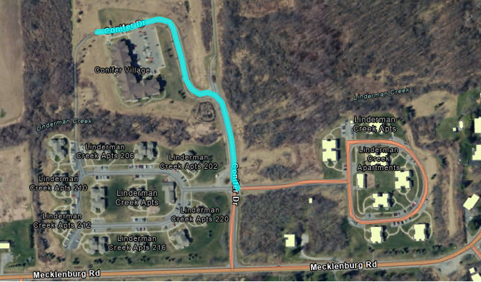
Whenever you come to a place where the road would change its name
(presumably at the corners), you want to finish one arc and start
another. Also, as much as possible, do each road as one line segment. To
easily identify the name of each road, you can add
Imagery Hybrid or Imagery with labels as
Basemap.
When finished, commit the changes. Your finished road should now be highlighted.
Merging Lines
Often when digitizing, we may want to merge several road segments together. To be able to see where one segment ends and another begins.
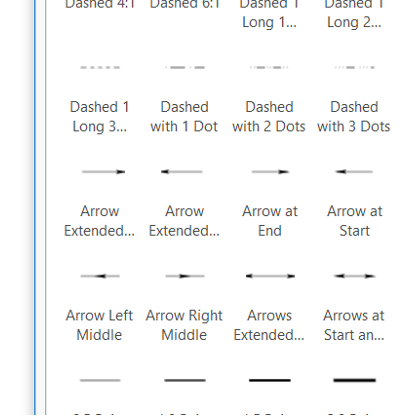
Change the line symbol for roadscl to the one called “arrows at start and end.”
If you want to merge two line segments, or a road that was done in
multiple pieces, select all the pieces with the select tool (hold shift
to select multiple features), and use the Merge
function
Edit toolbar to combine the parts into one arc (order
doesn’t matter, as none of the roads have attributes yet. This way you
can ensure that an entire road consists of only 1 segment.
Enter Attributes
Once the digitizing is done, you are ready to enter the attribute information for the roads.
Highlight the road you wish to edit and then open the attribute table.
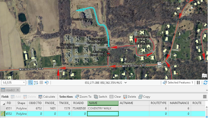
Since the editing session is still open, you should be able to edit the appropriate text columns directly (Name, etc.), assuming we know this information (you may have to refer to outside sources). We could then use this to label the streets. Finally, remember to save your edits.
Map 3: Create a map of the development (zoom in!) depicting your newly digitized roads (include the aerial basemap in the layout).
- Note: completing the circular road presents some difficulties, as you are not able to snap to a road segment you are currently editing. You may have to use multiple segments and then merge them together.
- Find out what these streets are called, edit the attribute information, and then include labels in your map.
Now it’s your turn!!!
Map 1: Map of the georeferenced historical map (including Coastline). (20 points)
- Please discuss some reasons why the historical map and the modern-day coastline do not line up more closely (maximum 100 words). (10 points)
Map 2: Map of the georeferenced CAD files. (20 points)
- Please include the aerial photograph (5 points) and coastline (5 points).
Map 3: Map of the completed, up to date roads. (20 points) - Please include the aerial image (5 points)
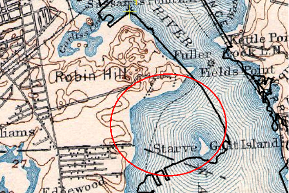
Map 4 (40 points): Go back to the Providence River project we were working on in the first part of the lab. Zoom to the area around the aerial photograph (the area between Robin Hill and Goat Island on the 1894 map).
- Create a new polygon layer, be sure to assign this polygon the appropriate coordinate system. (10 points)
- Digitize the land that has filled in the Providence River since 1894. (10 points)
- Use this polygon to calculate the total fill area. (10 points)
- Create a map layout that includes coastlines, the historical map as well as the new shapefile (use a transparent hatch fill). (10 points)
The END